Interpret Complex Linear Models with SHAP within Seconds

A linear model with complex interaction effects can be almost as opaque as a typical black-box like XGBoost.

XGBoost models are often interpreted with SHAP (Shapley Additive eXplanations): Each of e.g. 1000 randomly selected predictions is fairly decomposed into contributions of the features using the extremely fast TreeSHAP algorithm, providing a rich interpretation of the model as a whole. TreeSHAP was introduced in the Nature publication by Lundberg and Lee (2020).

Can we do the same for non-tree-based models like a complex GLM or a neural network? Yes, but we have to resort to slower model-agnostic SHAP algorithms:

• “fastshap” (Brandon Greenwell) implement an efficient version of the SHAP sampling approach by Erik Štrumbelj & Igor Kononenko (2014).
• “kernelshap” (Mayer and Watson) implements the Kernel SHAP algorithm by Lundberg and Lee (2017). It uses a constrained weighted regression to calculate the SHAP values of all features at the same time.

In the limit, the two algorithms provide the same SHAP values.

House prices

We will use a great dataset with 14’000 house prices sold in Miami in 2016. The dataset was kindly provided by Prof. Steven Bourassa for research purposes and can be found on OpenML.

The model

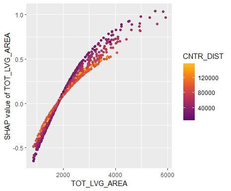
We will model house prices by a Gamma regression with log-link. The model includes factors, linear components and natural cubic splines. The relationship of living area and distance to central district is modeled by letting the spline bases of the two features interact.

library(OpenML)
library(tidyverse)
library(splines)
library(doFuture)
library(kernelshap)
library(shapviz)

raw <- OpenML::getOMLDataSet(43093)$data

# Lump rare level 3 and log transform the land size
prep <- raw %>%
  mutate(
    structure_quality = factor(structure_quality, labels = c(1, 2, 4, 4, 5)),
    log_landsize = log(LND_SQFOOT)
  )

# 1) Build model
xvars <- c("TOT_LVG_AREA", "log_landsize", "structure_quality",
           "CNTR_DIST", "age", "month_sold")

fit <- glm(
  SALE_PRC ~ ns(log(CNTR_DIST), df = 4) * ns(log(TOT_LVG_AREA), df = 4) +
    log_landsize + structure_quality + ns(age, df = 4) + ns(month_sold, df = 4),
  family = Gamma("log"),
  data = prep
)
summary(fit)

# Selected coefficients:
# log_landsize: 0.22559  
# structure_quality4: 0.63517305 
# structure_quality5: 0.85360956   

The model has 37 parameters. Some of the estimates are shown.

Interpretation

The workflow of a SHAP analysis is as follows:

1. Sample 1000 rows to explain
2. Sample 100 rows as background data used to estimate marginal expectations
3. Calculate SHAP values. This can be done fully in parallel by looping over the rows selected in Step 1
4. Analyze the SHAP values

Step 2 is the only additional step compared with TreeSHAP. It is required both for SHAP sampling values and Kernel SHAP.

# 1) Select rows to explain
set.seed(1)
X <- prep[sample(nrow(prep), 1000), xvars]

# 2) Select small representative background data
bg_X <- prep[sample(nrow(prep), 100), ]

# 3) Calculate SHAP values in fully parallel mode
registerDoFuture()
plan(multisession, workers = 6)  # Windows
# plan(multicore, workers = 6)   # Linux, macOS, Solaris

system.time( # <10 seconds
  shap_values <- kernelshap(
    fit, X, bg_X = bg_X, parallel = T, parallel_args = list(.packages = "splines")
  )
)

Thanks to parallel processing and some implementation tricks, we were able to decompose 1000 predictions within 10 seconds! By default, kernelshap() uses exact calculations up to eight features (exact regarding the background data), which would need an infinite amount of Monte-Carlo-sampling steps.

Note that glm() has a very efficient predict() function. GAMs, neural networks, random forests etc. usually take more time, e.g. 5 minutes to do the crunching.

Analyze the SHAP values

# 4) Analyze them
sv <- shapviz(shap_values)

sv_importance(sv, show_numbers = TRUE) +
  ggtitle("SHAP Feature Importance")

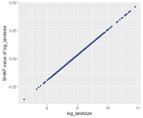
sv_dependence(sv, "log_landsize")
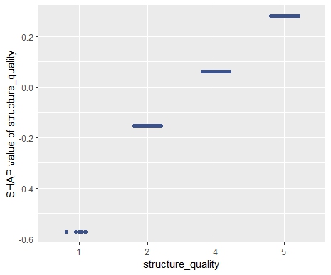
sv_dependence(sv, "structure_quality")
sv_dependence(sv, "age")
sv_dependence(sv, "month_sold")
sv_dependence(sv, "TOT_LVG_AREA", color_var = "auto")
sv_dependence(sv, "CNTR_DIST", color_var = "auto")

# Slope of log_landsize: 0.2255946
diff(sv$S[1:2, "log_landsize"]) / diff(sv$X[1:2, "log_landsize"])

# Difference between structure quality 4 and 5: 0.2184365
diff(sv$S[2:3, "structure_quality"])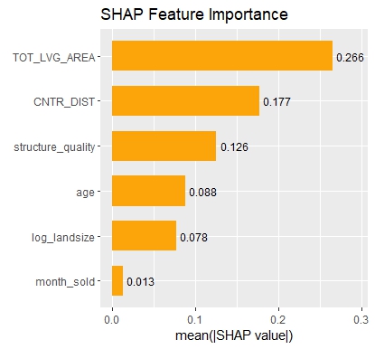

Summary

• Interpreting complex linear models with SHAP is an option. There seems to be a correspondence between regression coefficients and SHAP dependence, at least for additive components.
• Kernel SHAP in R is fast. For models with slower predict() functions (e.g. GAMs, random forests, or neural nets), we often need to wait a couple of minutes.

The complete R script can be found here.