Lost in Translation between R and Python 9
This is the next article in our series “Lost in Translation between R and Python”. The aim of this series is to provide high-quality R and Python code to achieve some non-trivial tasks. If you are to learn R, check out the R tab below. Similarly, if you are to learn Python, the Python tab will be your friend.
Kernel SHAP
SHAP is one of the most used model interpretation technique in Machine Learning. It decomposes predictions into additive contributions of the features in a fair way. For tree-based methods, the fast TreeSHAP algorithm exists. For general models, one has to resort to computationally expensive Monte-Carlo sampling or the faster Kernel SHAP algorithm. Kernel SHAP uses a regression trick to get the SHAP values of an observation with a comparably small number of calls to the predict function of the model. Still, it is much slower than TreeSHAP.
Two good references for Kernel SHAP:
- Scott M. Lundberg and Su-In Lee. A Unified Approach to Interpreting Model Predictions. Advances in Neural Information Processing Systems 30, 2017.
- Ian Covert and Su-In Lee. Improving KernelSHAP: Practical Shapley Value Estimation Using Linear Regression. Proceedings of The 24th International Conference on Artificial Intelligence and Statistics, PMLR 130:3457-3465, 2021.
In our last post, we introduced our new “kernelshap” package in R. Since then, the package has been substantially improved, also by the big help of David Watson:
- The package now supports multi-dimensional predictions.
- It received a massive speed-up
- Additionally, parallel computing can be activated for even faster calculations.
- The interface has become more intuitive.
- If the number of features is small (up to ten or eleven), it can provide exact Kernel SHAP values just like the reference Python implementation.
- For a larger number of features, it now uses partly-exact (“hybrid”) calculations, very similar to the logic in the Python implementation.
With those changes, the R implementation is about to meet the Python version at eye level.
Example with four features
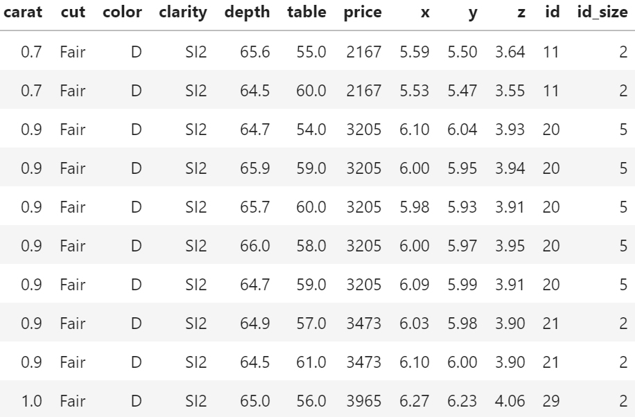
In the following, we use the diamonds data to fit a linear regression with
- log(price) as response
- log(carat) as numeric feature
- clarity, color and cut as categorical features (internally dummy encoded)
- interactions between log(carat) and the other three “C” variables. Note that the interactions are very weak
Then, we calculate SHAP decompositions for about 1000 diamonds (every 53th diamond), using 120 diamonds as background dataset. In this case, both R and Python will use exact calculations based on m=2^4 – 2 = 14 possible binary on-off vectors (a value of 1 representing a feature value picked from the original observation, a value of 0 a value picked from the background data).
library(ggplot2)
library(kernelshap)
# Turn ordinal factors into unordered
ord <- c("clarity", "color", "cut")
diamonds[, ord] <- lapply(diamonds[ord], factor, ordered = FALSE)
# Fit model
fit <- lm(log(price) ~ log(carat) * (clarity + color + cut), data = diamonds)
# Subset of 120 diamonds used as background data
bg_X <- diamonds[seq(1, nrow(diamonds), 450), ]
# Subset of 1018 diamonds to explain
X_small <- diamonds[seq(1, nrow(diamonds), 53), c("carat", ord)]
# Exact KernelSHAP (5 seconds)
system.time(
ks <- kernelshap(fit, X_small, bg_X = bg_X)
)
ks
# SHAP values of first 2 observations:
# carat clarity color cut
# [1,] -2.050074 -0.28048747 0.1281222 0.01587382
# [2,] -2.085838 0.04050415 0.1283010 0.03731644
# Using parallel backend
library("doFuture")
registerDoFuture()
plan(multisession, workers = 2) # Windows
# plan(multicore, workers = 2) # Linux, macOS, Solaris
# 3 seconds on second call
system.time(
ks3 <- kernelshap(fit, X_small, bg_X = bg_X, parallel = TRUE)
)
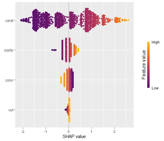
# Visualization
library(shapviz)
sv <- shapviz(ks)
sv_importance(sv, "bee")import numpy as np import pandas as pd from plotnine.data import diamonds from statsmodels.formula.api import ols from shap import KernelExplainer # Turn categoricals into integers because, inconveniently, kernel SHAP # requires numpy array as input ord = ["clarity", "color", "cut"] x = ["carat"] + ord diamonds[ord] = diamonds[ord].apply(lambda x: x.cat.codes) X = diamonds[x].to_numpy() # Fit model with interactions and dummy variables fit = ols( "np.log(price) ~ np.log(carat) * (C(clarity) + C(cut) + C(color))", data=diamonds ).fit() # Background data (120 rows) bg_X = X[0:len(X):450] # Define subset of 1018 diamonds to explain X_small = X[0:len(X):53] # Calculate KernelSHAP values ks = KernelExplainer( model=lambda X: fit.predict(pd.DataFrame(X, columns=x)), data = bg_X ) sv = ks.shap_values(X_small) # 74 seconds sv[0:2] # array([[-2.05007406, -0.28048747, 0.12812216, 0.01587382], # [-2.0858379 , 0.04050415, 0.12830103, 0.03731644]])
The results match, hurray!
Example with nine features
The computation effort of running exact Kernel SHAP explodes with the number of features. For nine features, the number of relevant on-off vectors is 2^9 – 2 = 510, i.e. about 36 times larger than with four features.
We now modify above example, adding five additional features to the model. Note that the model structure is completely non-sensical. We just use it to get a feeling about what impact a 36 times larger workload has.
Besides exact calculations, we use an almost exact hybrid approach for both R and Python, using 126 on-off vectors (p*(p+1) for the exact part and 4p for the sampling part, where p is the number of features), resulting in a significant speed-up both in R and Python.
fit <- lm(
  log(price) ~ log(carat) * (clarity + color + cut) + x + y + z + table + depth,
  data = diamonds
)

# Subset of 1018 diamonds to explain
X_small <- diamonds[seq(1, nrow(diamonds), 53), setdiff(names(diamonds), "price")]

# Exact Kernel SHAP: 61 seconds
system.time(
  ks <- kernelshap(fit, X_small, bg_X = bg_X, exact = TRUE)
)
ks
#          carat        cut     color     clarity         depth         table          x           y            z
# [1,] -1.842799 0.01424231 0.1266108 -0.27033874 -0.0007084443  0.0017787647 -0.1720782 0.001330275 -0.006445693
# [2,] -1.876709 0.03856957 0.1266546  0.03932912 -0.0004202636 -0.0004871776 -0.1739880 0.001397792 -0.006560624

# Default, using an almost exact hybrid algorithm: 17 seconds
system.time(
  ks <- kernelshap(fit, X_small, bg_X = bg_X, parallel = TRUE)
)
#          carat        cut     color     clarity         depth         table          x           y            z
# [1,] -1.842799 0.01424231 0.1266108 -0.27033874 -0.0007084443  0.0017787647 -0.1720782 0.001330275 -0.006445693
# [2,] -1.876709 0.03856957 0.1266546  0.03932912 -0.0004202636 -0.0004871776 -0.1739880 0.001397792 -0.006560624
x = ["carat"] + ord + ["table", "depth", "x", "y", "z"]
X = diamonds[x].to_numpy()

# Fit model with interactions and dummy variables
fit = ols(
  "np.log(price) ~ np.log(carat) * (C(clarity) + C(cut) + C(color)) + table + depth + x + y + z",
  data=diamonds
).fit()

# Background data (120 rows)
bg_X = X[0:len(X):450]

# Define subset of 1018 diamonds to explain
X_small = X[0:len(X):53]

# Calculate KernelSHAP values: 12 minutes
ks = KernelExplainer(
  model=lambda X: fit.predict(pd.DataFrame(X, columns=x)),
  data = bg_X
)
sv = ks.shap_values(X_small)
sv[0:2]
# array([[-1.84279897e+00, -2.70338744e-01,  1.26610769e-01,
#          1.42423108e-02,  1.77876470e-03, -7.08444295e-04,
#         -1.72078182e-01,  1.33027467e-03, -6.44569296e-03],
#        [-1.87670887e+00,  3.93291219e-02,  1.26654599e-01,
#          3.85695742e-02, -4.87177593e-04, -4.20263565e-04,
#         -1.73988040e-01,  1.39779179e-03, -6.56062359e-03]])

# Now, using a hybrid between exact and sampling: 5 minutes
sv = ks.shap_values(X_small, nsamples=126)
sv[0:2]
# array([[-1.84279897e+00, -2.70338744e-01,  1.26610769e-01,
#          1.42423108e-02,  1.77876470e-03, -7.08444295e-04,
#         -1.72078182e-01,  1.33027467e-03, -6.44569296e-03],
#        [-1.87670887e+00,  3.93291219e-02,  1.26654599e-01,
#          3.85695742e-02, -4.87177593e-04, -4.20263565e-04,
#         -1.73988040e-01,  1.39779179e-03, -6.56062359e-03]])
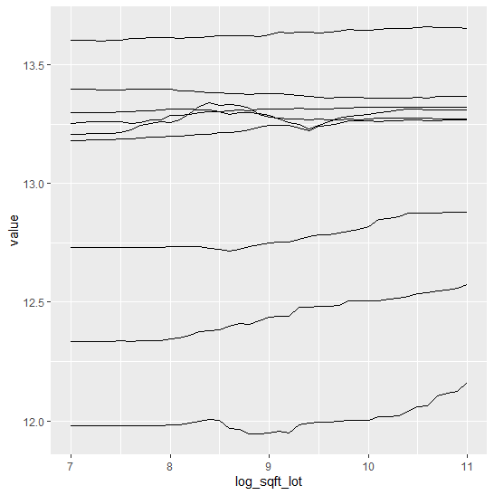
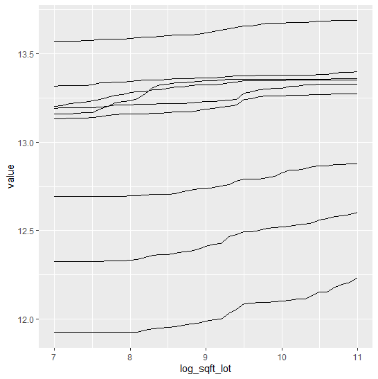
Again, the results are essentially the same between R and Python, but also between the hybrid algorithm and the exact algorithm. This is interesting, because the hybrid algorithm is significantly faster than the exact one.
Wrap-Up
- R is catching up with Python’s superb “shap” package.
- For two non-trivial linear regressions with interactions, the “kernelshap” package in R provides the same output as Python.
- The hybrid between exact and sampling KernelSHAP (as implemented in Python and R) offers a very good trade-off between speed and accuracy.
kernelshap()in R is fast!
The Python and R codes can be found here:
The examples were run on a Windows notebook with an Intel i7-8650U 4 core CPU.