Lost in Translation between R and Python 7
Hello random forest friends
This is the next article in our series “Lost in Translation between R and Python”. The aim of this series is to provide high-quality R and Python 3 code to achieve some non-trivial tasks. If you are to learn R, check out the R tab below. Similarly, if you are to learn Python, the Python tab will be your friend.
Monotonic constraints
On ML competition platforms like Kaggle, complex and unintuitively behaving models dominate. In this respect, reality is completely different. There, the majority of models do not serve as pure prediction machines but rather as fruitful source of information. Furthermore, even if used as prediction machine, the users of the models might expect a certain degree of consistency when “playing” with input values.
A classic example are statistical house appraisal models. An additional bathroom or an additional square foot of ground area is expected to raise the appraisal, everything else being fixed (ceteris paribus). The user might lose trust in the model if the opposite happens.
One way to enforce such consistency is to monitor the signs of coefficients of a linear regression model. Another useful strategy is to impose monotonicity constraints on selected model effects.
Trees and monotonic constraints
Monotonicity constraints are especially simple to implement for decision trees. The rule is basically as follows:
If a monotonicity constraint would be violated by a split on feature X, it is rejected. (Or a large penalty is subtracted from the corresponding split gain.) This will imply monotonic behavior of predictions in X, keeping all other features fixed.
Tree ensembles like boosted trees or random forests will automatically inherit this property.
Boosted trees
Most implementations of boosted trees offer monotonicity constraints. Here is a selection:
- R & Python: XGBoost
- R & Python: LightGBM
- R & Python: CatBoost
- Python: Scikit-Learn histogram gradient booster
- R: gbm
What about random forests?
Unfortunately, the picture is completely different for random forests. At the time of writing, I am not aware of any random forest implementation in R or Python offering this useful feature.
Some options
- Implement monotonic constrainted random forests from scratch.
- Ask for this feature in existing implementations.
- Be creative and use XGBoost to emulate random forests.
For the moment, let’s stick to option 3. In our last R <-> Python blog post, we demonstrated that XGBoost’s random forest mode works essentially as good as standard random forest implementations, at least in regression settings and using sensible defaults.
Warning: Be careful with imposing monotonicity constraints
Ask yourself: does the constraint really make sense for all possible values of other features? You will see that the answer is often “no”.
An example: If your house price model uses the features “number of rooms” and “living area”, then a monotonic constraint on “living area” might make sense (given any number of rooms), while such constraint would be non-sensical for the number of rooms. Why? Because having six rooms in a 1200 square feet home is not necessarily better than having just five rooms in an equally sized home.
Let’s try it out
We use a nice dataset containing information on over 20,000 sold houses in Kings County. Along with the sale price, different features describe the size and location of the properties. The dataset is available on OpenML.org with ID 42092.
The following R and Python codes
- fetch the data,
- prepare the ML setting,
- fit unconstrained XGBoost random forests using log sales price as response,
- and visualize the effect of log ground area by individual conditional expectation (ICE) curves.
An ICE curve for variable X shows how the prediction of one specific observation changes if the value of X changes. Repeating this for multiple observations gives an idea of the effect of X. The average over multiple ICE curves produces the famous partial dependent plot.
library(farff)
library(OpenML)
library(dplyr)
library(xgboost)
set.seed(83454)
rmse <- function(y, pred) {
sqrt(mean((y-pred)^2))
}
# Load King Country house prices dataset on OpenML
# ID 42092, https://www.openml.org/d/42092
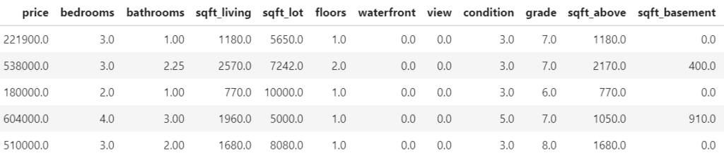
df <- getOMLDataSet(data.id = 42092)$data
head(df)
# Prepare
df <- df %>%
mutate(
log_price = log(price),
log_sqft_lot = log(sqft_lot),
year = as.numeric(substr(date, 1, 4)),
building_age = year - yr_built,
zipcode = as.integer(as.character(zipcode))
)
# Define response and features
y <- "log_price"
x <- c("grade", "year", "building_age", "sqft_living",
"log_sqft_lot", "bedrooms", "bathrooms", "floors", "zipcode",
"lat", "long", "condition", "waterfront")
# random split
ix <- sample(nrow(df), 0.8 * nrow(df))
y_test <- df[[y]][-ix]
# Fit untuned, but good(!) XGBoost random forest
dtrain <- xgb.DMatrix(data.matrix(df[ix, x]),
label = df[ix, y])
params <- list(
objective = "reg:squarederror",
learning_rate = 1,
num_parallel_tree = 500,
subsample = 0.63,
colsample_bynode = 1/3,
reg_lambda = 0,
max_depth = 20,
min_child_weight = 2
)
system.time( # 25 s
unconstrained <- xgb.train(
params,
data = dtrain,
nrounds = 1,
verbose = 0
)
)
pred <- predict(unconstrained, data.matrix(df[-ix, x]))
# Test RMSE: 0.172
rmse(y_test, pred)
# ICE curves via our flashlight package
library(flashlight)
pred_xgb <- function(m, X) predict(m, data.matrix(X[, x]))
fl <- flashlight(
model = unconstrained,
label = "unconstrained",
data = df[ix, ],
predict_function = pred_xgb
)
light_ice(fl, v = "log_sqft_lot", indices = 1:9,
evaluate_at = seq(7, 11, by = 0.1)) %>%
plot()# Imports
import numpy as np
from sklearn.datasets import fetch_openml
from sklearn.model_selection import train_test_split
from sklearn.metrics import mean_squared_error
from sklearn.inspection import PartialDependenceDisplay
from xgboost import XGBRFRegressor
# Fetch data from OpenML
df = fetch_openml(data_id=42092, as_frame=True)["frame"]
# Prepare data
df = df.assign(
year=lambda x: x.date.str[0:4].astype(int),
zipcode=lambda x: x.zipcode.astype(int),
log_sqft_lot=lambda x: np.log(x.sqft_lot),
building_age=lambda x: x.year - x.yr_built,
)
# Feature list
xvars = [
"grade",
"year",
"building_age",
"sqft_living",
"log_sqft_lot",
"bedrooms",
"bathrooms",
"floors",
"zipcode",
"lat",
"long",
"condition",
"waterfront",
]
# Data split
y_train, y_test, X_train, X_test = train_test_split(
np.log(df["price"]), df[xvars], train_size=0.8, random_state=766
)
# Modeling - wall time: 39 seconds
param_dict = dict(
n_estimators=500,
max_depth=20,
learning_rate=1,
subsample=0.63,
colsample_bynode=1 / 3,
reg_lambda=0,
objective="reg:squarederror",
min_child_weight=2,
)
unconstrained = XGBRFRegressor(**param_dict).fit(X_train, y_train)
# Test RMSE 0.176
pred = unconstrained.predict(X_test)
print(f"RMSE: {mean_squared_error(y_test, pred, squared=False):.03f}")
# ICE and PDP - wall time: 47 seconds
PartialDependenceDisplay.from_estimator(
unconstrained,
X=X_train,
features=["log_sqft_lot"],
kind="both",
subsample=20,
random_state=1,
)
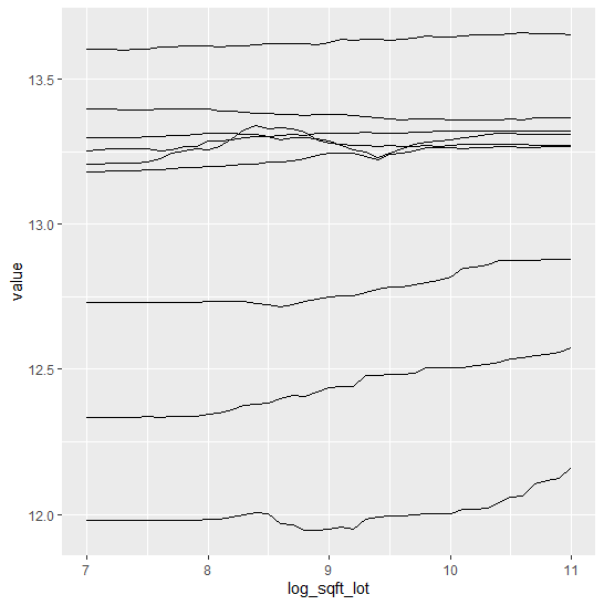
We clearly see many non-monotonic (and in this case counterintuitive) ICE curves.
What would a model give with monotonically increasing constraint on the ground area?
# Monotonic increasing constraint
(params$monotone_constraints <- 1 * (x == "log_sqft_lot"))

system.time( #  179s
  monotonic <- xgb.train(
    params,
    data = dtrain,
    nrounds = 1,
    verbose = 0
  )
)

pred <- predict(monotonic, data.matrix(df[-ix, x]))

# Test RMSE: 0.176
rmse(y_test, pred)

fl_m <- flashlight(
  model = monotonic,
  label = "monotonic",
  data = df[ix, ],
  predict_function = pred_xgb
)

light_ice(fl_m, v = "log_sqft_lot", indices = 1:9,
          evaluate_at = seq(7, 11, by = 0.1)) %>%
  plot()
# One needs to pass the constraints as single string, which is rather ugly
mc = "(" + ",".join([str(int(x == "log_sqft_lot")) for x in xvars]) + ")"
print(mc)
# Modeling - wall time 49 seconds
constrained = XGBRFRegressor(monotone_constraints=mc, **param_dict)
constrained.fit(X_train, y_train)
# Test RMSE: 0.178
pred = constrained.predict(X_test)
print(f"RMSE: {mean_squared_error(y_test, pred, squared=False):.03f}")
# ICE and PDP - wall time 39 seconds
PartialDependenceDisplay.from_estimator(
constrained,
X=X_train,
features=["log_sqft_lot"],
kind="both",
subsample=20,
random_state=1,
)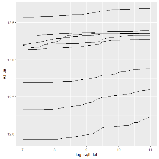
We see:
- It works! Each ICE curve in log(lot area) is monotonically increasing. This means that predictions are monotonically increasing in lot area, keeping all other feature values fixed.
- The model performance is slightly worse. This is the price paid for receiving a more intuitive behaviour in an important feature.
- In Python, both models take about the same time to fit (30-40 s on a 4 core i7 CPU laptop). Curiously, in R, the constrained model takes about six times longer to fit than the unconstrained one (170 s vs 30 s).
Summary
- Monotonic constraints help to create intuitive models.
- Unfortunately, as per now, native random forest implementations do not offer such constraints.
- Using XGBoost’s random forest mode is a temporary solution until native random forest implementations add this feature.
- Be careful to add too many constraints: does a constraint really make sense for all other (fixed) choices of feature values?
The Python notebook and R code can be found at:
Leave a Reply