Let’s explain a {tidymodels} random forest by classic explainability methods (permutation importance, partial dependence plots (PDP), Friedman’s H statistics), and also fancy SHAP.
Disclaimer: {hstats}, {kernelshap} and {shapviz} are three of my own packages.
Diabetes data
We will use the diabetes prediction dataset of Kaggle to model diabetes (yes/no) as a function of six demographic features (age, gender, BMI, hypertension, heart disease, and smoking history). It has 100k rows.
Note: The data additionally contains the typical diabetes indicators HbA1c level and blood glucose level, but we wont use them to avoid potential causality issues, and to gain insights also for people that do not know these values.
R
# https://www.kaggle.com/datasets/iammustafatz/diabetes-prediction-dataset
library(tidyverse)
library(tidymodels)
library(hstats)
library(kernelshap)
library(shapviz)
library(patchwork)
df0 <- read.csv("diabetes_prediction_dataset.csv") # from above Kaggle link
dim(df0) # 100000 9
head(df0)
# gender age hypertension heart_disease smoking_history bmi HbA1c_level blood_glucose_level diabetes
# Female 80 0 1 never 25.19 6.6 140 0
# Female 54 0 0 No Info 27.32 6.6 80 0
# Male 28 0 0 never 27.32 5.7 158 0
# Female 36 0 0 current 23.45 5.0 155 0
# Male 76 1 1 current 20.14 4.8 155 0
# Female 20 0 0 never 27.32 6.6 85 0
summary(df0)
anyNA(df0) # FALSE
table(df0$smoking_history, useNA = "ifany")
# DATA PREPARATION
# Note: tidymodels needs a factor response for classification
df1 <- df0 |>
transform(
y = factor(diabetes, levels = 0:1, labels = c("No", "Yes")),
female = (gender == "Female") * 1,
smoking_history = factor(
smoking_history,
levels = c("No Info", "never", "former", "not current", "current", "ever")
),
bmi = pmin(bmi, 50)
)
# UNIVARIATE ANALYSIS
ggplot(df1, aes(diabetes)) +
geom_bar(fill = "chartreuse4")
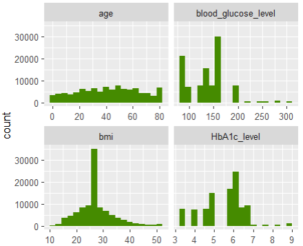
df1 |>
select(age, bmi, HbA1c_level, blood_glucose_level) |>
pivot_longer(everything()) |>
ggplot(aes(value)) +
geom_histogram(fill = "chartreuse4", bins = 19) +
facet_wrap(~ name, scale = "free_x")
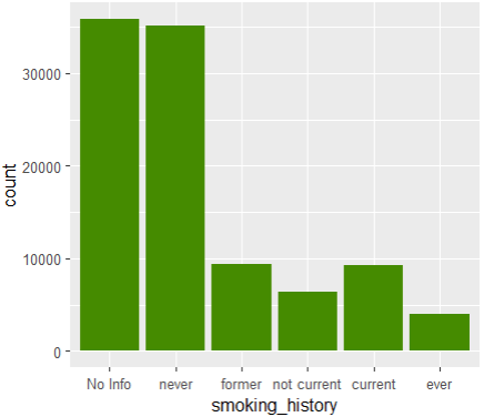
ggplot(df1, aes(smoking_history)) +
geom_bar(fill = "chartreuse4")
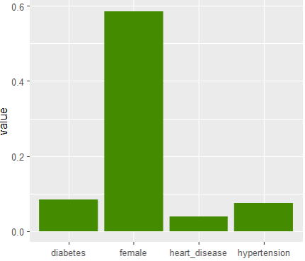
df1 |>
select(heart_disease, hypertension, female) |>
pivot_longer(everything()) |>
ggplot(aes(name, value)) +
stat_summary(fun = mean, geom = "bar", fill = "chartreuse4") +
xlab(element_blank())
Modeling
Let’s fit a random forest via tidymodels with {ranger} backend.
We add a predict function pf() that outputs only the probability of the “Yes” class.
set.seed(1)
ix <- initial_split(df1, strata = diabetes, prop = 0.8)
train <- training(ix)
test <- testing(ix)

xvars <- c("age", "bmi", "smoking_history", "heart_disease", "hypertension", "female")

rf_spec <- rand_forest(trees = 500) |>
  set_mode("classification") |>
  set_engine("ranger", num.threads = NULL, seed = 49)

rf_wf <- workflow() |>
  add_model(rf_spec) |>
  add_formula(reformulate(xvars, "y"))

model <- rf_wf |>
    fit(train)

# predict() gives No/Yes columns
predict(model, head(test), type = "prob")
# .pred_No .pred_Yes
#    0.981    0.0185

# We need to extract only the "Yes" probabilities
pf <- function(m, X) {
  predict(m, X, type = "prob")$.pred_Yes
}
pf(model, head(test))  # 0.01854290 ...
Classic explanation methods
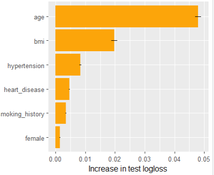
# 4 times repeated permutation importance wrt test logloss
imp <- perm_importance(
model, X = test, y = "diabetes", v = xvars, pred_fun = pf, loss = "logloss"
)
plot(imp) +
xlab("Increase in test logloss")
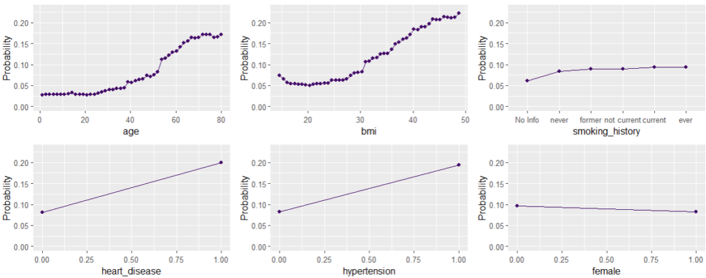
# Partial dependence of age
partial_dep(model, v = "age", train, pred_fun = pf) |>
plot()
# All PDP in one patchwork
p <- lapply(xvars, function(x) plot(partial_dep(model, v = x, X = train, pred_fun = pf)))
wrap_plots(p) &
ylim(0, 0.23) &
ylab("Probability")
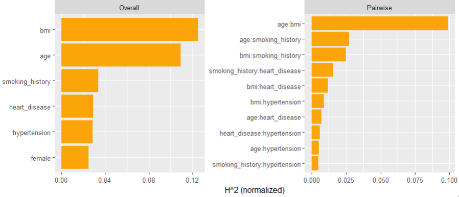
# Friedman's H stats
system.time( # 20 s
H <- hstats(model, train[xvars], approx = TRUE, pred_fun = pf)
)
H # 15% of prediction variability comes from interactions
plot(H)
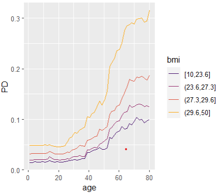
# Stratified PDP of strongest interaction
partial_dep(model, "age", BY = "bmi", X = train, pred_fun = pf) |>
plot(show_points = FALSE)Feature importance
Permutation importance measures by how much the average test loss (in our case log loss) increases when a feature is shuffled before calculating the losses. We repeat the process four times and also show standard errors.
Main effects
Main effects are estimated by PDP. They show how the average prediction changes with a feature, keeping every other feature fixed. Using a fixed vertical axis helps to grasp the strenght of the effect.
Interaction strength
Interaction strength can be measured by Friedman’s H statistics, see the earlier blog post. A specific interaction can then be visualized by a stratified PDP.
SHAP
What insights does a SHAP analysis bring?
We will crunch slow exact permutation SHAP values via kernelshap::permshap(). If we had more features, we could switch to
kernelshap::kernelshap()- Brandon Greenwell’s {fastshap}, or to the
- {treeshap} package of my colleages from TU Warsaw.
set.seed(1)
X_explain <- train[sample(1:nrow(train), 1000), xvars]
X_background <- train[sample(1:nrow(train), 200), ]
system.time( # 10 minutes
shap_values <- permshap(model, X = X_explain, bg_X = X_background, pred_fun = pf)
)
shap_values <- shapviz(shap_values)
shap_values # 'shapviz' object representing 1000 x 6 SHAP matrix
saveRDS(shap_values, file = "shap_values.rds")
# shap_values <- readRDS("shap_values.rds")
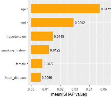
sv_importance(shap_values, show_numbers = TRUE)
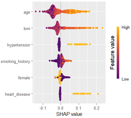
sv_importance(shap_values, kind = "bee")
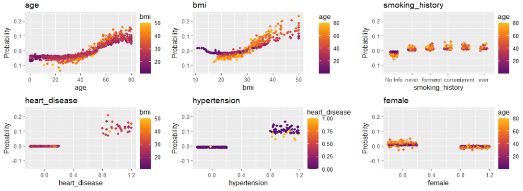
sv_dependence(shap_values, v = xvars) &
ylim(-0.14, 0.24) &
ylab("Probability")SHAP importance
SHAP “summary” plot
SHAP dependence plots
Final words
- {hstats}, {kernelshap} and {shapviz} can explain any model with XAI methods like permutation importance, PDPs, Friedman’s H, and SHAP. This, obviously, also includes models developed with {tidymodels}.
- They would actually even work for multi-output models, e.g., classification with more than two categories.
- Studying a blackbox with XAI methods is always worth the effort, even if the methods have their issues. I.e., an imperfect explanation is still better than no explanation.
- Model-agnostic SHAP takes a little bit of time, but it is usually worth the effort.
Leave a Reply