What makes a ML model a black-box? It is the interactions. Without any interactions, the ML model is additive and can be exactly described.
Studying interaction effects of ML models is challenging. The main XAI approaches are:
- Looking at ICE plots, stratified PDP, and/or 2D PDP.
- Study vertical scatter in SHAP dependence plots, or even consider SHAP interaction values.
- Check partial-dependence based H-statistics introduced in Friedman and Popescu (2008), or related statistics.
This post is mainly about the third approach. Its beauty is that we get information about all interactions. The downside: it is as good/bad as partial dependence functions. And: the statistics are computationally very expensive to compute (of order n^2).
Different R packages offer some of these H-statistics, including {iml}, {gbm}, {flashlight}, and {vivid}. They all have their limitations. This is why I wrote the new R package {hstats}:
- It is very efficient.
- Has a clean API. DALEX explainers and meta-learners (mlr3, Tidymodels, caret) work out-of-the-box.
- Supports multivariate predictions, including classification models.
- Allows to calculate unnormalized H-statistics. They help to compare pairwise and three-way statistics.
- Contains fast multivariate ICE/PDPs with optional grouping variable.
In Python, there is the very interesting project artemis. I will write a post on it later.
Statistics supported by {hstats}
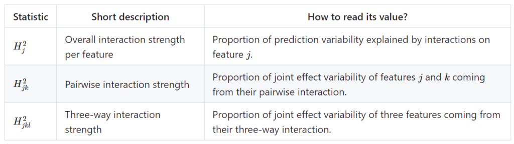
Furthermore, a global measure of non-additivity (proportion of prediction variability unexplained by main effects), and a measure of feature importance is available. For technical details and references, check the following pdf or github.
Classification example
Let’s fit a probability random forest on iris species.
library(ranger)
library(ggplot2)
library(hstats)
v <- setdiff(colnames(iris), "Species")
fit <- ranger(Species ~ ., data = iris, probability = TRUE, seed = 1)
s <- hstats(fit, v = v, X = iris) # 8 seconds run-time
s
# Proportion of prediction variability unexplained by main effects of v:
# setosa versicolor virginica
# 0.002705945 0.065629375 0.046742035
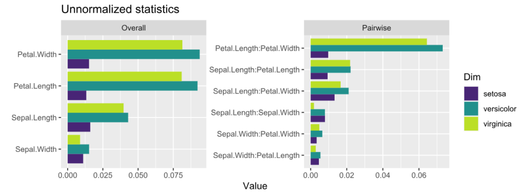
plot(s, normalize = FALSE, squared = FALSE) +
ggtitle("Unnormalized statistics") +
scale_fill_viridis_d(begin = 0.1, end = 0.9)
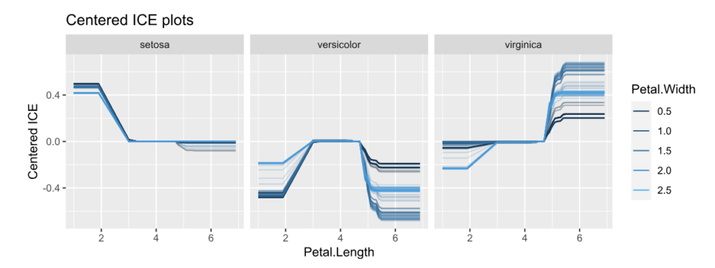
ice(fit, v = "Petal.Length", X = iris, BY = "Petal.Width", n_max = 150) |>
plot(center = TRUE) +
ggtitle("Centered ICE plots")
Interpretation:
- The features with strongest interactions are Petal Length and Petal Width. These interactions mainly affect species “virginica” and “versicolor”. The effect for “setosa” is almost additive.
- Unnormalized pairwise statistics show that the strongest absolute interaction happens indeed between Petal Length and Petal Width.
- The centered ICE plots shows how the interaction manifests: The effect of Petal Length heavily depends on Petal Width, except for species “setosa”. Would a SHAP analysis show the same?
DALEX example
Here, we consider a random forest regression on “Sepal.Length”.
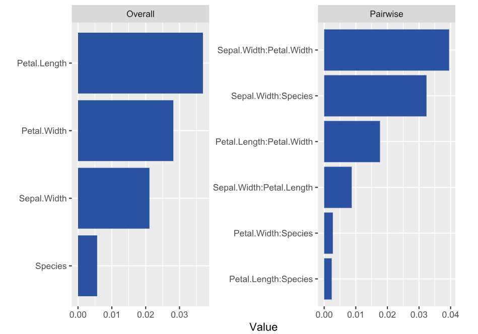
library(DALEX)
library(ranger)
library(hstats)

set.seed(1)

fit <- ranger(Sepal.Length ~ ., data = iris)
ex <- explain(fit, data = iris[-1], y = iris[, 1])

s <- hstats(ex)  # 2 seconds
s  # Non-additivity index 0.054
plot(s)
plot(ice(ex, v = "Sepal.Width", BY = "Petal.Width"), center = TRUE)
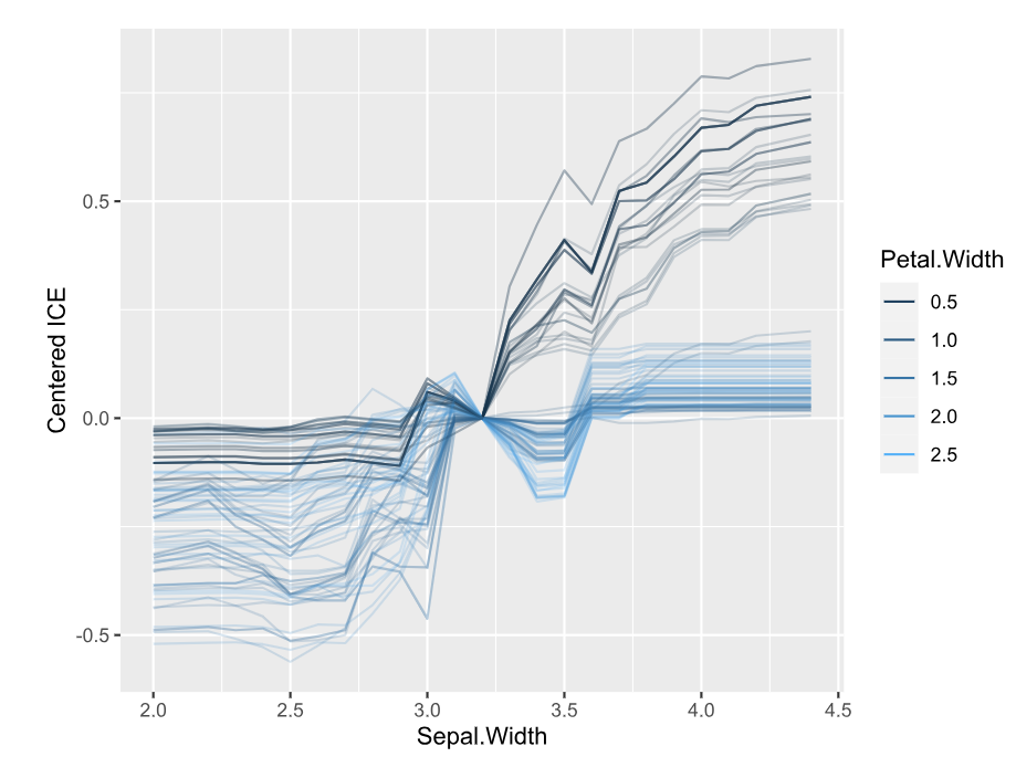
Interpretation
- Petal Length and Width show the strongest overall associations. Since we are considering normalized statistics, we can say: “About 3.5% of prediction variability comes from interactions with Petal Length”.
- The strongest relative pairwise interaction happens between Sepal Width and Petal Width: Again, because we study normalized H-statistics, we can say: “About 4% of total prediction variability of the two features Sepal Width and Petal Width can be attributed to their interactions.”
- Overall, all interactions explain only about 5% of prediction variability (see text output).
Try it out!
The complete R script can be found here. More examples and background can be found on the Github page of the project.
Leave a Reply