In our latest post, we explained how to use ML + XAI to build strong generalized linear models with R. Let’s do the same with Python.
Insurance pricing data
We will use again a synthetic dataset with 1 Mio insurance policies, with reference:
Mayer, M., Meier, D. and Wuthrich, M.V. (2023),
SHAP for Actuaries: Explain any Model.
https://doi.org/10.2139/ssrn.4389797
Let’s start by loading and describing the data:
import numpy as np
import pandas as pd
import matplotlib.pyplot as plt
import seaborn as sns
import shap
from sklearn.datasets import fetch_openml
from sklearn.inspection import PartialDependenceDisplay
from sklearn.metrics import mean_poisson_deviance
from sklearn.dummy import DummyRegressor
from lightgbm import LGBMRegressor
# We need preview version of glum that adds formulaic API
# !pip install git+https://github.com/Quantco/glum@glum-v3#egg=glum
from glum import GeneralizedLinearRegressor
# Load data
df = fetch_openml(data_id=45106, parser="pandas").frame
df.head()
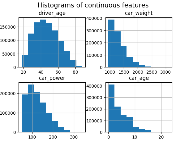
# Continuous features
df.hist(["driver_age", "car_weight", "car_power", "car_age"])
_ = plt.suptitle("Histograms of continuous features", fontsize=15)
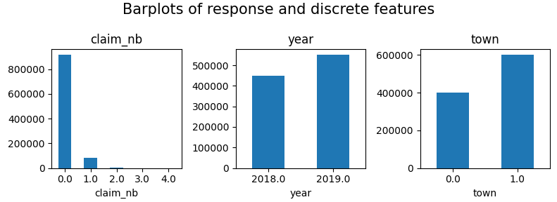
# Response and discrete features
fig, axes = plt.subplots(figsize=(8, 3), ncols=3)
for v, ax in zip(["claim_nb", "year", "town"], axes):
df[v].value_counts(sort=False).sort_index().plot(kind="bar", ax=ax, rot=0, title=v)
plt.suptitle("Barplots of response and discrete features", fontsize=15)
plt.tight_layout()
plt.show()
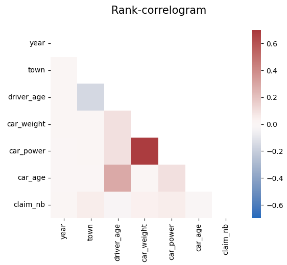
# Rank correlations
corr = df.corr("spearman")
mask = np.triu(np.ones_like(corr, dtype=bool))
plt.suptitle("Rank-correlogram", fontsize=15)
_ = sns.heatmap(
corr, mask=mask, vmin=-0.7, vmax=0.7, center=0, cmap="vlag", square=True
)
Modeling
- We fit a tuned Boosted Trees model to model log(E(claim count)) via Poisson deviance loss.
- And perform a SHAP analysis to derive insights.
from sklearn.model_selection import train_test_split

X_train, X_test, y_train, y_test = train_test_split(
    df.drop("claim_nb", axis=1), df["claim_nb"], test_size=0.1, random_state=30
)

# Tuning step not shown. Number of boosting rounds found via early stopping on CV performance
params = dict(
    learning_rate=0.05,
    objective="poisson",
    num_leaves=7,
    min_child_samples=50,
    min_child_weight=0.001,
    colsample_bynode=0.8,
    subsample=0.8,
    reg_alpha=3,
    reg_lambda=5,
    verbose=-1,
)

model_lgb = LGBMRegressor(n_estimators=360, **params)
model_lgb.fit(X_train, y_train)

# SHAP analysis
X_explain = X_train.sample(n=2000, random_state=937)
explainer = shap.Explainer(model_lgb)
shap_val = explainer(X_explain)

plt.suptitle("SHAP importance", fontsize=15)
shap.plots.bar(shap_val)

for s in [shap_val[:, 0:3], shap_val[:, 3:]]:
    shap.plots.scatter(s, color=shap_val, ymin=-0.5, ymax=1)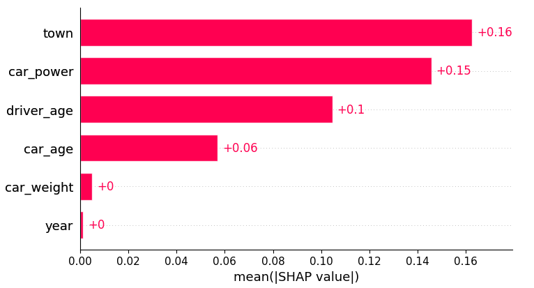
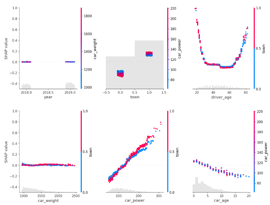
Here, we would come to the conclusions:
car_weightandyearmight be dropped, depending on the specify aim of the model.- Add a regression spline for
driver_age. - Add an interaction between
car_powerandtown.
Build strong GLM
Let’s build a GLM with these insights. Two important things:
- Glum is an extremely powerful GLM implementation that was inspired by a pull request of our Christian Lorentzen.
- In the upcoming version 3.0, it adds a formula API based of formulaic, a very performant formula parser. This gives a very easy way to add interaction effects, regression splines, dummy encodings etc.
model_glm = GeneralizedLinearRegressor(
family="poisson",
l1_ratio=1.0,
alpha=1e-10,
formula="car_power * C(town) + bs(driver_age, 7) + car_age",
)
model_glm.fit(X_train, y=y_train) # 1 second on old laptop
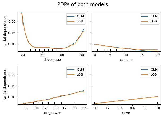
# PDPs of both models
fig, ax = plt.subplots(2, 2, figsize=(7, 5))
cols = ("tab:blue", "tab:orange")
for color, name, model in zip(cols, ("GLM", "LGB"), (model_glm, model_lgb)):
disp = PartialDependenceDisplay.from_estimator(
model,
features=["driver_age", "car_age", "car_power", "town"],
X=X_explain,
ax=ax if name == "GLM" else disp.axes_,
line_kw={"label": name, "color": color},
)
fig.suptitle("PDPs of both models", fontsize=15)
fig.tight_layout()
# Stratified PDP of car_power
for color, town in zip(("tab:blue", "tab:orange"), (0, 1)):
mask = X_explain.town == town
disp = PartialDependenceDisplay.from_estimator(
model_glm,
features=["car_power"],
X=X_explain[mask],
ax=None if town == 0 else disp.axes_,
line_kw={"label": town, "color": color},
)
plt.suptitle("PDP of car_power stratified by town (0 vs 1)", fontsize=15)
_ = plt.ylim(0, 0.2)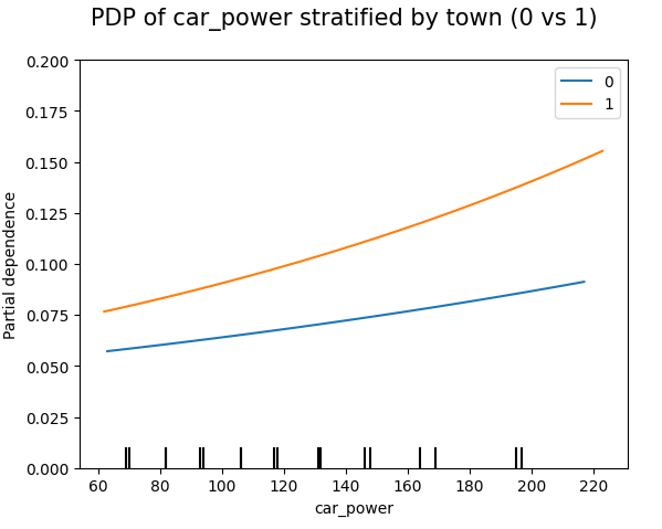
In this relatively simple situation, the mean Poisson deviance of our models are very simlar now:
model_dummy = DummyRegressor().fit(X_train, y=y_train)
deviance_null = mean_poisson_deviance(y_test, model_dummy.predict(X_test))

dev_imp = []
for name, model in zip(("GLM", "LGB", "Null"), (model_glm, model_lgb, model_dummy)):
    dev_imp.append((name, mean_poisson_deviance(y_test, model.predict(X_test))))
pd.DataFrame(dev_imp, columns=["Model", "Mean_Poisson_Deviance"])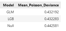
Final words
- Glum is an extremely powerful GLM implementation – we have only scratched its surface. You can expect more blogposts on Glum…
- Having a formula interface is especially useful for adding interactions. Fingers crossed that the upcoming version 3.0 will soon be released.
- Building GLMs via ML + XAI is so smooth, especially when you work with large data. For small data, you need to be careful to not add hidden overfitting to the model.
Leave a Reply