SHAP (SHapley Additive exPlanations, Lundberg and Lee, 2017) is an ingenious way to study black box models. SHAP values decompose – as fair as possible – predictions into additive feature contributions.
When it comes to SHAP, the Python implementation is the de-facto standard. It not only offers many SHAP algorithms, but also provides beautiful plots. In R, the situation is a bit more confusing. Different packages contain implementations of SHAP algorithms, e.g.,
some of which with great visualizations. Plus there is SHAPforxgboost (see my recent post), originally designed to visualize the results of SHAP values calculated from XGBoost, but it can also be used more generally by now.
The shapviz package
In order to entangle calculation from visualization, the shapviz package was designed. It solely focuses on visualization of SHAP values. Closely following its README, it currently provides these plots:
sv_waterfall(): Waterfall plots to study single predictions.sv_force(): Force plots as an alternative to waterfall plots.sv_importance(): Importance plots (bar and/or beeswarm plots) to study variable importance.sv_dependence(): Dependence plots to study feature effects (optionally colored by heuristically strongest interacting feature).
They require a “shapviz” object, which is built from two things only:
S: Matrix of SHAP valuesX: Dataset with corresponding feature values
Furthermore, a “baseline” can be passed to represent an average prediction on the scale of the SHAP values.
A key feature of the “shapviz” package is that X is used for visualization only. Thus it is perfectly fine to use factor variables, even if the underlying model would not accept these.
To further simplify the use of shapviz, direct connectors to the packages
are available.
Installation
The package shapviz can be installed from CRAN or Github:
devtools::install_github("shapviz")
devtools::install_github("mayer79/shapviz")
Example
Shiny diamonds… let’s model their prices by four “c” variables with XGBoost, and create an explanation dataset with 2000 randomly picked diamonds.
library(shapviz)
library(ggplot2)
library(xgboost)

set.seed(3653)

X <- diamonds[c("carat", "cut", "color", "clarity")]
dtrain <- xgb.DMatrix(data.matrix(X), label = diamonds$price)

fit <- xgb.train(
  params = list(learning_rate = 0.1, objective = "reg:squarederror"),
  data = dtrain,
  nrounds = 65L
)

# Explanation dataset
X_small <- X[sample(nrow(X), 2000L), ]
Create “shapviz” object
One line of code creates a shapviz object. It contains SHAP values and feature values for the set of observations we are interested in. Note again that X is solely used as explanation dataset, not for calculating SHAP values.
In this example we construct the shapviz object directly from the fitted XGBoost model. Thus we also need to pass a corresponding prediction dataset X_pred used for calculating SHAP values by XGBoost.
shp <- shapviz(fit, X_pred = data.matrix(X_small), X = X_small)
Explaining one single prediction
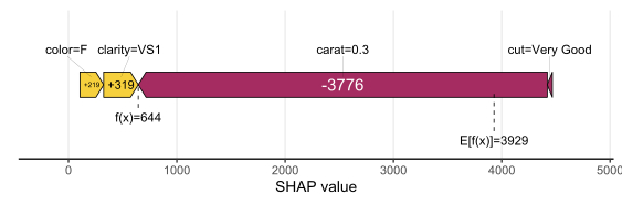
Let’s start by explaining a single prediction by a waterfall plot or, alternatively, a force plot.
# Two types of visualizations
sv_waterfall(shp, row_id = 1)
sv_force(shp, row_id = 1
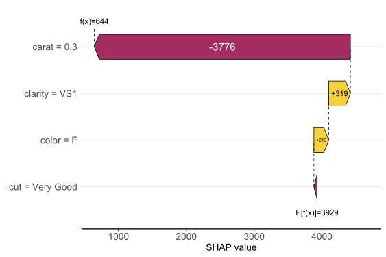
Factor/character variables are kept as they are, even if the underlying XGBoost model required them to be integer encoded.
Explaining the model as a whole
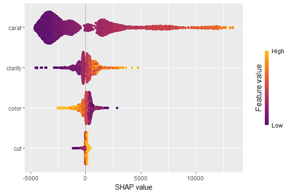
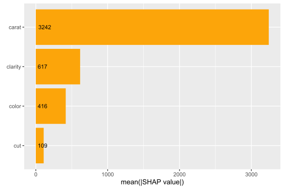
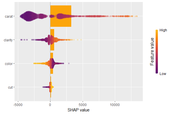
We have decomposed 2000 predictions, not just one. This allows us to study variable importance at a global model level by studying average absolute SHAP values as a bar plot or by looking at beeswarm plots of SHAP values.
# Three types of variable importance plots
sv_importance(shp)
sv_importance(shp, kind = "bar")
sv_importance(shp, kind = "both", alpha = 0.2, width = 0.2)
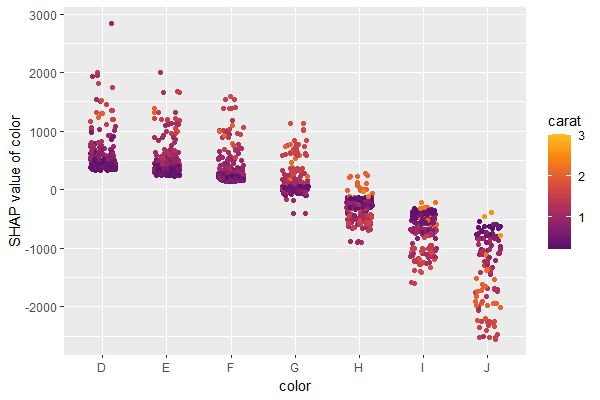
A scatterplot of SHAP values of a feature like color against its observed values gives a great impression on the feature effect on the response. Vertical scatter gives additional info on interaction effects. shapviz offers a heuristic to pick another feature on the color scale with potential strongest interaction.
sv_dependence(shp, v = "color", "auto")
Summary
- The “shapviz” has a single purpose: making SHAP plots.
- Its interface is optimized for existing SHAP crunching packages and can easily be used in future packages as well.
- All plots are highly customizable. Furthermore, they are all written with
ggplotand allow corresponding modifications.
The complete R script can be found here.
References
Scott M. Lundberg and Su-In Lee. A Unified Approach to Interpreting Model Predictions. Advances in Neural Information Processing Systems 30 (2017).