Category: Linear Algebra

  • Histograms, Gradient Boosted Trees, Group-By Queries and One-Hot Encoding

    This post shows how filling histograms can be done in very different ways thereby connecting very different areas: from gradient boosted trees to SQL queries to one-hot encoding. Let’s jump into it!

    Modern gradient boosted trees (GBT) like LightGBM, XGBoost and the HistGradientBoostingRegressor of scikit-learn all use two techniques on top of standard gradient boosting:

    • 2nd order Taylor expansion of the loss which amounts to using gradients and hessians.
    • One histogram per feature: bin the feature and fill the histogram with the gradients and hessians.

    The filling of the histograms is often the bottleneck when fitting GBTs. While filling a single histogram is very fast, this operation is executed many times: for each boosting round, for each tree split and for each feature. This is the reason why GBT implementations have dedicated routines for it. We look into this operation from different angles.

    For the coming (I)Python code snippets to work (# %% indicates a new notebook cell), we need the following imports.

    import duckdb                    # v0.5.1
    import matplotlib.pyplot as plt  # v.3.6.1
    from matplotlib.ticker import MultipleLocator
    import numpy as np               # v1.23.4
    import pandas as pd              # v1.5.0
    import pyarrow as pa             # v9.0.0
    import tabmat                    # v3.1.2
    
    from sklearn.ensemble._hist_gradient_boosting.histogram import (
        _build_histogram_root,
    )                                # v1.1.2
    from sklearn.ensemble._hist_gradient_boosting.common import (
      HISTOGRAM_DTYPE
    )

    Naive Histogram Visualisation

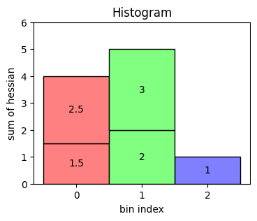
    As a starter, we create a small table with two columns: bin index and value of the hessian.

    def highlight(df):
        if df["bin"] == 0:
            return ["background-color: rgb(255, 128, 128)"] * len(df)
        elif df["bin"] == 1:
            return ["background-color: rgb(128, 255, 128)"] * len(df)
        else:
            return ['background-color: rgb(128, 128, 255)'] * len(df)
    
    df = pd.DataFrame({"bin": [0, 2, 1, 0, 1], "hessian": [1.5, 1, 2, 2.5, 3]})
    df.style.apply(highlight, axis=1)
      bin hessian
    0 0 1.500000
    1 2 1.000000
    2 1 2.000000
    3 0 2.500000
    4 1 3.000000

    A histogram then sums up all the hessian values belonging to the same bin. The result looks like the following.

    Above table visualised as histogram

    Dedicated Method

    We simulate filling the histogram of a single feature. Therefore, we draw 1,000,000 random variables for gradients and hessians as well as the bin indices.

    import duckdb
    import pyarrow as pa
    import numpy as np
    import tabmat
    
    from sklearn.ensemble._hist_gradient_boosting.histogram import (
        _build_histogram_root,
    )
    from sklearn.ensemble._hist_gradient_boosting.common import HISTOGRAM_DTYPE
    
    
    rng = np.random.default_rng(42)
    n_obs = 1000_000
    n_bins = 256
    binned_feature = rng.integers(0, n_bins, size=n_obs, dtype=np.uint8)
    gradients = rng.normal(size=n_obs).astype(np.float32)
    hessians = rng.lognormal(size=n_obs).astype(np.float32)

    Now we use the dedicated (and private!) and single-threaded method _build_histogram_root from sckit-learn to fill a histogram.

    hist_root = np.zeros((1, n_bins), dtype=HISTOGRAM_DTYPE)
    %time _build_histogram_root(0, binned_feature, gradients, hessians, hist_root)
    # Wall time: 1.38 ms

    This executes in around 1.4 ms. This is quite fast. But again, imagine 100 boosting rounds with 10 tree splits on average and 100 features. This means this is done around 100,000 times and would therefore take roughly 2 minutes.

    Let’s have a look at the first 5 bins:

    hist_root[:, 0:5]
    array([[(-79.72386998, 6508.89500265, 3894),
            ( 37.98393589, 6460.63222205, 3998),
            ( 53.54256977, 6492.22722797, 3805),
            ( 21.19542398, 6797.34159299, 3928),
            ( 16.24716742, 6327.03757573, 3875)]],
          dtype=[('sum_gradients', '<f8'), ('sum_hessians', '<f8'), ('count', '<u4')])

    SQL Group-By Query

    Someone familiar with SQL and database queries might immediately see how this task can be formulated as SQL group-by-aggregate query. To demonstrate it on our simulated data, we use DuckDB as well as Apache Arrow (the file format as well as the Python library pyarrow). You can read more about DuckDB in our post DuckDB: Quacking SQL.

    # %%
    con = duckdb.connect()
    arrow_table = pa.Table.from_pydict(
        {
            "bin": binned_feature,
            "gradients": gradients,
            "hessians": hessians,
    })
    # Read data once to make timing fairer
    arrow_result = con.execute("SELECT * FROM arrow_table")
    
    # %%
    %%time
    arrow_result = con.execute("""
    SELECT
        bin as bin,
        SUM(gradients) as sum_gradients,
        SUM(hessians) as sum_hessians,
        COUNT() as count
    FROM arrow_table
    GROUP BY bin
    """).arrow()
    # Wall time: 6.52 ms

    On my laptop, this takes about 6.5 ms and, upon sorting, gives the same results:

    arrow_result.sort_by("bin").slice(length=5)
    pyarrow.Table
    bin: uint8
    sum_gradients: double
    sum_hessians: double
    count: int64
    ----
    bin: [[0,1,2,3,4]]
    sum_gradients: [[-79.72386997545254,37.98393589106854,53.54256977112527,21.195423980039777,16.247167424764484]]
    sum_hessians: [[6508.895002648234,6460.632222048938,6492.227227974683,6797.341592986137,6327.037575732917]]
    count: [[3894,3998,3805,3928,3875]]

    As we have the table as an Arrow table, we can stay within pyarrow:

    %%time
    arrow_result = arrow_table.group_by("bin").aggregate(
        [
            ("gradients", "sum"),
            ("hessians", "sum"),
            ("bin", "count"),
        ]
    )
    # Wall time: 10.8 ms

    The fact that DuckDB is faster than Arrow on this task might have to do with the large invested effort on parallelised group-by operations, see their post Parallel Grouped Aggregation in DuckDB for more infos.

    One-Hot encoded Matrix Multiplication

    I think it is very interesting that filling histograms can be written as a matrix multiplication! The trick is to view the feature as a categorical feature and use its one-hot encoded matrix representation. This blows up memory, of course. Note that one-hot encoding is usually met with generalized linear models (GLM) in order to incorporate nominal categorical feature variables with no internal ordering in the design matrix.

    For our demonstration, we use a numpy index trick to construct the one-hot encoded matrix employing the fact that the binned feature already contains the right indices.

    # %%
    %%time
    m_OHE = np.eye(n_bins)[binned_feature].T
    vec = np.column_stack((gradients, hessians, np.ones_like(gradients)))
    # Wall time: 770 ms
    
    # %%
    %time result_ohe = m_OHE @ vec
    # Wall time: 199 ms
    
    # %%
    result_ohe[:5]
    array([[ -79.72386998, 6508.89500265, 3894.        ],
           [  37.98393589, 6460.63222205, 3998.        ],
           [  53.54256977, 6492.22722797, 3805.        ],
           [  21.19542398, 6797.34159299, 3928.        ],
           [  16.24716742, 6327.03757573, 3875.        ]])

    This is way slower, but, somehow surprisingly, produces the same result.

    The one-hot encoded matrix is very sparse, with only one non-zero value per column, i.e. only one out of 256 (number of bins) values is non-zero. This structure can be exploited to reduce both CPU time as well as memory consumption, with the help of the package tabmat that was built to accelerate GLMs. Unfortunately, tabmat only provides a matrix-vector multiplication (and the sandwich product, of course), but no matrix-matrix multiplication. So we have to do a little extra work.

    # %%
    %time m_categorical = tabmat.CategoricalMatrix(cat_vec=binned_feature)
    # Wall time: 21.5 ms
    
    # %%
    # tabmat needs contigous arrays with dtype = Python float = float64
    vec = np.asfortranarray(vec, dtype=float)
    
    # %%
    %%time
    tabmat_result = np.column_stack(
        (
            vec[:, 0] @ m_categorical,
            vec[:, 1] @ m_categorical,
            vec[:, 2] @ m_categorical,
        )
    )
    # Wall time: 4.82 ms
    
    # %%
    tabmat_result[0:5]
    array([[ -79.72386998, 6508.89500265, 3894.        ],
           [  37.98393589, 6460.63222205, 3998.        ],
           [  53.54256977, 6492.22722797, 3805.        ],
           [  21.19542398, 6797.34159299, 3928.        ],
           [  16.24716742, 6327.03757573, 3875.        ]])

    While the timing of this approach is quite good, the construction of a CategoricalMatrix requires more time than the matrix-vector multiplication.

    Conclusion

    In the end, the special (Cython) routine of scikit-learn ist the fastest of our tested methods for filling histograms. The other GBT libraries have their own even more specialised routines which might be a reason for even faster fit times. What we learned in this post is that this seemingly simple task plays a very crucial part in modern GBTs and can be accomplished by very different approaches. These different approaches uncover connections of algorithms of quite different domains.

    The full code as ipython notebook can be found at https://github.com/lorentzenchr/notebooks/blob/master/blogposts/2022-10-31%20histogram-GBT-GroupBy-OHE.ipynb.

  • From Least Squares Benchmarks to the Marchenko–Pastur Distribution

    In this blog post, I tell the story how I learned about a theorem for random matrices of the two Ukrainian🇺🇦 mathematicians Vladimir Marchenko and Leonid Pastur. It all started with benchmarking least squares solvers in scipy.

    Setting the Stage for Least Squares Solvers

    Least squares starts with a matrix A \in \mathbb{R}^{n,p} and a vector b \in \mathbb{R}^{n} and one is interested in solution vectors x \in \mathbb{R}^{p} fulfilling

    x^\star = \argmin_x ||Ax-b||_2^2 \,.

    You can read more about least squares in our earlier post Least Squares Minimal Norm Solution. There are many possible ways to tackle this problem and many algorithms are available. One standard solver is LSQR with the following properties:

    • Iterative solver, which terminates when some stopping criteria are smaller than a user specified tolerance.
    • It only uses matrix-vector products. Therefore, it is suitable for large and sparse matrices A.
    • It effectively solves the normal equations A^T A = A^Tb based on a bidiagonalization procedure of Golub and Kahan (so never really calculating A^T A).
    • It is, unfortunately, susceptible to ill-conditioned matrices A, which we demonstrated in our earlier post.

    Wait, what is an ill-conditioned matrix? This is most easily explained with the help of the singular value decomposition (SVD). Any real valued matrix permits a decomposition into three parts:

    A = U S V^T \,.

    U and V are orthogonal matrices, but not of further interest to us. The matrix S on the other side is (rectangular) diagonal with only non-negative entries s_i = S_{ii} \geq 0. A matrix A is said to be ill-conditioned if it has a large condition number, which can be defined as the ratio of largest and smallest singular value, \mathrm{cond}(A) = \frac{\max_i s_i}{\min_i s_i} = \frac{s_{\mathrm{max}}}{s_{\mathrm{min}}}. Very often, large condition numbers make numerical computations difficult or less precise.

    Benchmarking LSQR

    One day, I decided to benchmark the computation time of least squares solvers provided by scipy, in particular LSQR. I wanted results for different sizes n, p of the matrix dimensions. So I needed to somehow generate different matrices A. There are a myriad ways to do that. Naive as I was, I did the most simple thing and used standard Normal (Gaussian) distributed random matrices A_{ij} \sim \mathcal{N}(0, 1) and ran benchmarks on those. Let’s see how that looks in Python.

    from collections import OrderedDict
    from functools import partial
    
    import matplotlib.pyplot as plt
    import numpy as np
    from scipy.linalg import lstsq
    from scipy.sparse.linalg import lsqr
    import seaborn as sns
    from neurtu import Benchmark, delayed
    
    plt.ion()
    
    p_list = [100, 500]
    rng = np.random.default_rng(42)
    X = rng.standard_normal(max(p_list) ** 2 * 2)
    y = rng.standard_normal(max(p_list) * 2)
    
    def bench_cases():    
        for p in p_list:
            for n in np.arange(0.1, 2.1, 0.1):
                n = int(p*n)
                A = X[:n*p].reshape(n, p)
                b = y[:n]
                for solver in ['lstsq', 'lsqr']:
                    tags = OrderedDict(n=n, p=p, solver=solver)
                    if solver == 'lstsq':
                        solve = delayed(lstsq, tags=tags)
                    elif solver == 'lsqr':
                        solve = delayed(
                            partial(
                                lsqr, atol=1e-10, btol=1e-10, iter_lim=1e6
                            ),
                            tags=tags)
    
                    yield solve(A, b)
    
    bench = Benchmark(wall_time=True)
    df = bench(bench_cases())
    
    g = sns.relplot(x='n', y='wall_time', hue='solver', col='p',
                kind='line', facet_kws={'sharex': False, 'sharey': False},
                data=df.reset_index(), marker='o')
    g.set_titles("p = {col_name}")
    g.set_axis_labels("n", "Wall time (s)")
    g.set(xscale="linear", yscale="log")
    
    plt.subplots_adjust(top=0.9)
    g.fig.suptitle('Benchmark LSQR vs LSTSQ')
    for ax in g.axes.flatten():
        ax.tick_params(labelbottom=True)
    Timing benchmark of LSQR and standard LAPACK LSTSQ solvers for different sizes of n on the x-axis and p=100 left, p=500 right.

    The left plot already looks a bit suspicious around n=p. But what is happening on the right side? Where does this spike of LSQR come from? And why does the standard least squares solver, SVD-based lstsq, not show this spike?

    When I saw these results, I thought something might be wrong with LSQR and opened an issue on the scipy github repository, see https://github.com/scipy/scipy/issues/11204. The community there is really fantastic. Brett Naul pointed me to ….

    The Marchenko–Pastur Distribution

    The Marchenko–Pastur distribution is the distribution of the eigenvalues (singular values of square matrices) of certain random matrices in the large sample limit. Given a random matrix A \in \mathbb{R}^{n,p} with i.i.d. entries A_{ij} having zero mean, \mathbb{E}[A_{ij}] = 0, and finite variance, \mathrm{Var}[A_{ij}] = \sigma^2 < \infty, we define the matrix Y_n = \frac{1}{n}A^T A \in \mathbb{R}^{p,p}. As square and even symmetric matrix, Y_n has a simpler SVD, namely Y_n = V \Sigma V^T. One can in fact show that V is the same as in the SVD of A and that the diagonal matrix \Sigma = \frac{1}{n}S^TS contains the squared singular values of A and \min(0, p-n) extra zero values. The (diagonal) values of \Sigma are called eigenvalues \lambda_1, \ldots, \lambda_p of Y_n. Note/ that the eigenvalues are themselves random variables, and we are interested in their probability distribution or probability measure. We define the (random) measure \mu_p(B) = \frac{1}{p} \#\{\lambda_j \in B\} for all intervals B \subset \mathbb{R}.

    The theorem of Marchenko and Pastur then states that for n, p \rightarrow \infty with \frac{p}{n} \rightarrow \rho , we have \mu_p \rightarrow \mu, where

    \mu(B) = \begin{cases} (1-\frac{1}{\rho})\mathbb{1}_{0\in B} + \nu(B),\quad &\rho > 1 \\ \nu(B), \quad & 0\leq\rho\leq 1 \end{cases} \,,
    \nu(x) = \frac{1}{2\pi\sigma^2} \frac{\sqrt{(\rho_+ - x)(x - \rho_-)}}{\rho x} \mathbb{1}_{x \in [\rho_-, \rho_+]} dx\,,
    \rho_{\pm} = \sigma^2 (1\pm\sqrt{\rho})^2 \,.

    We can at least derive the point mass at zero for \rho>1 \Leftrightarrow p>n: We said above that \Sigma contains p-n extra zeros and those correspond to a density of \frac{p-n}{p}=1 – \frac{1}{\rho} at zero.

    A lot of math so far. Just note that the assumptions on A are exactly met by the one in our benchmark above. Also note that the normal equations can be expressed in terms of Y_n as n Y_n x = A^Tb.

    Empirical Confirmation of the Marchenko–Pastur Distribution

    Before we come back to the spikes in our benchmark, let us have a look and see how good the Marchenko–Pastur distribution is approximated for finite sample size. We choose n=1000, p=500 which gives \rho=\frac{1}{2}. We plot a histrogram of the eigenvalues next to the Marchenko–Pastur distribution.

    def marchenko_pastur_mu(x, rho, sigma2=1):
        x = np.atleast_1d(x).astype(float)
        rho_p = sigma2 * (1 + np.sqrt(rho)) ** 2
        rho_m = sigma2 * (1 - np.sqrt(rho)) ** 2
        mu = np.zeros_like(x)
        is_nonzero = (rho_m < x) & (x < rho_p)
        x_valid = x[is_nonzero]
        factor = 1 / (2 * np.pi * sigma2 * rho)
        mu[is_nonzero] = factor / x_valid
        mu[is_nonzero] *= np.sqrt((rho_p - x_valid) * (x_valid - rho_m))
        if rho > 1:
            mu[x == 0] = 1 - 1 / rho
        return mu
    
    fig, ax = plt.subplots()
    
    n, p = 1000, 500
    A = X.reshape(n, p)
    Y = 1/n * A.T @ A
    eigenvals, _ = np.linalg.eig(Y)
    ax.hist(eigenvals.real, bins=50, density=True, label="histogram")
    x = np.linspace(0, np.max(eigenvals.real), 100)
    ax.plot(x, marchenko_pastur_mu(x, rho=p/n), label="MP distribution")
    ax.legend()
    ax.set_xlabel("eigenvalue")
    ax.set_ylabel("probability")
    ax.set_title("Empirical evidence for n=1000, p=500, rho=0.5")
    Hitogram of eigenvalues for n=100, p=500 versus Marchenko–Pastur distribution

    I have to say, I am very impressed by this good agreement for n=1000, which is far from being huge.

    Conclusion

    Let’s visualize the Marchenko–Pastur distribution Y_n for several ratios \rho and fix \sigma=1:

    fig, ax = plt.subplots()
    
    rho_list = [0.5, 1, 1.5]
    x = np.linspace(0, 5, 1000)[1:] # exclude 0
    for rho in rho_list:
        y = marchenko_pastur_mu(x, rho)
        line, = ax.plot(x, y, label=f"rho={rho}")
        # plot zero point mass
        if rho > 1:
            ax.scatter(0, marchenko_pastur_mu(0, rho), color = line.get_color())
    
    ax.set_ylim(None, 1.2)
    ax.legend()
    ax.set_title("Marchenko-Pastur Distribution")
    ax.set_xlabel("x")
    ax.set_ylabel("dmu/dx")
    Marchenko-Pastur distribution for several ratios rho. The green dot is the point mass at zero.

    From this figure it becomes obvious that the closer the ratio \rho = 1, the higher the probability for very tiny eigenvalues. This results in a high probability for an ill-conditioned matrix A^TA coming from an ill-conditioned matrix A. Let’s confirm that:

    p = 500
    n_vec = []
    c_vec = []
    for n in np.arange(0.1, 2.05, 0.05):
        n = int(p*n)
        A = X[:n*p].reshape(n, p)
        n_vec.append(n)
        c_vec.append(np.linalg.cond(A))
    
    fig, ax = plt.subplots()
    ax.plot(n_vec, c_vec)
    ax.set_xlabel("n")
    ax.set_ylabel("condition number of A")
    ax.set_title("Condition Number of A for p=500")
    Condition number of the random matrix A

    As a result of the ill-conditioned A, the LSQR solver has problems to achieve its tolerance criterion, needs more iterations, and takes longer time. This is exactly what we observed in the benchmark plots: the peak occurred around n=p. The SVD-based lstsq solver, on the other hand, does not use an iterative scheme and does not need more time for ill-conditioned matrices.

    You find the accompanying notebook here: https://github.com/lorentzenchr/notebooks/blob/master/blogposts/2022-05-22%20from%20least%20squares%20benchmarks%20to%20the%20marchenko-pastur%20distribution.ipynb

  • Least Squares Minimal Norm Solution

    Least squares is a cornerstone of linear algebra, optimization and therefore also for statistical and machine learning models. Given a matrix A ∈ Rn,p and a vector b ∈ Rn, we search for

    x^\star = \argmin_{x \in R^p} ||Ax - b||^2

    Translation for regression problems: Search for coefficients β→x given the design or features matrix X→A and target y→b.

    In the case of a singular matrix A or an underdetermined setting n<p, the above definition is not precise and permits many solutions x⋆. In those cases, a more precise definition is the minimum norm solution of least squares:

    x^\star = \argmin_{x} ||x||^2
    \quad \text{subject to} \quad
    \min_{x \in R^p} ||Ax - b||^2

    In words: We solve the least squares problem and choose the solution with minimal Euclidean norm.

    We will show step by step what this means on a series on overdetermined systems. In linear regression with more observations than features, n>p, one says the system is overdetermined, leading to ||Ax^\star-b||^2 > 0 in most cases.

    Regular System

    Let’s start with a well-behaved example. To have good control over the matrix, we construct it by its singular value decomposition (SVD) A=USV’ with orthogonal matrices U and V and diagonal matrix S. Recall that S has only non-negative entries and — for regular matrices — even strictly positive values. Therefore, we start by setting \operatorname{diag}(S) = (1, 2, 3, 4, 5).

    from pprint import pprint
    import matplotlib.pyplot as plt
    import numpy as np
    from numpy.linalg import norm
    from scipy.stats import ortho_group
    from scipy import linalg
    from scipy.sparse import linalg as spla
    
    
    def generate_U_S_Vt(n=10, p=5, random_state=532):
        """Generate SVD to construct a regular matrix A.
        
        A has n rows, p columns.
        
        Returns
        -------
        U: orthogonal matrix
        S: diagonal matrix
        Vt: orthogonal matrix
        """
        r = min(n, p)
        S = np.diag(1.0 * np.arange(1, 1 + r))
        if n > p:
            # add rows with value 0
            S = np.concatenate((S, np.zeros((n - p, p))), axis=0)
        elif p > n:
            # add columns with value 0
            S = np.concatenate((S, np.zeros((n, p - n))), axis=1)
        U = ortho_group.rvs(n, random_state=random_state)
        Vt = ortho_group.rvs(p, random_state=random_state + 1)
        return U, S, Vt
    
    
    def solve_least_squares(A, b):
        """Solve least squares with several methods.
        
        Returns
        ------
        x : dictionary with solver and solution
        """
        x = {}
        x["gelsd"] = linalg.lstsq(A, b, lapack_driver="gelsd")[0]
        x["gelsy"] = linalg.lstsq(A, b, lapack_driver="gelsy")[0]
        x["lsqr"] = spla.lsqr(A, b)[0]
        x["lsmr"] = spla.lsmr(A, b)[0]
        x["normal_eq"] = linalg.solve(A.T @ A, A.T @ b, assume_a="sym")
    
        return x
    
    
    def print_dict(d):
        np.set_string_function(np.array2string)
        pprint(d)
        np.set_string_function(None)
    
    
    np.set_printoptions(precision=5)
    
    
    n = 10
    p = 5
    
    U, S, Vt = generate_U_S_Vt(n=n, p=p)
    A = U @ S @ Vt
    
    x_true = np.round(6 * Vt.T[:p, 0])  # interesting choice
    rng = np.random.default_rng(157)
    noise = rng.standard_normal(n)
    b = A @ x_true + noise
    
    S_inv = np.copy(S.T)
    S_inv[S_inv>0] = 1/S_inv[S_inv>0]
    
    x_exact = Vt.T @ S_inv @ U.T @ b
    
    print(f"x_exact = {x_exact}")
    print_dict(solve_least_squares(A, b))
    x_exact = [ 0.78087 -4.74942 -0.99938 -2.38327 -3.7431 ] {'gelsd': [ 0.78087 -4.74942 -0.99938 -2.38327 -3.7431 ],  'gelsy': [ 0.78087 -4.74942 -0.99938 -2.38327 -3.7431 ],  'lsmr': [ 0.78087 -4.74942 -0.99938 -2.38327 -3.7431 ],  'lsqr': [ 0.78087 -4.74942 -0.99938 -2.38327 -3.7431 ],  'normal_eq': [ 0.78087 -4.74942 -0.99938 -2.38327 -3.7431 ]}

    We see that all least squares solvers do well on regular systems, be it the LAPACK routines for direct least squares, GELSD and GELSY, the iterative solvers LSMR and LSQR or solving the normal equations by the LAPACK routine SYSV for symmetric matrices.

    Singular System

    We convert our regular matrix in a singular one by setting its first diagonal element to zero.

    S[0, 0] = 0
    A = U @ S @ Vt
    
    S_inv = np.copy(S.T)
    S_inv[S_inv>0] = 1/S_inv[S_inv>0]
    
    # Minimum Norm Solution
    x_exact = Vt.T @ S_inv @ U.T @ b
    
    print(f"x_exact = {x_exact}")
    x_solution = solve_least_squares(A, b)
    print_dict(x_solution)
    x_exact = [-0.21233  0.00708  0.34973 -0.30223 -0.0235 ] {'gelsd': [-0.21233  0.00708  0.34973 -0.30223 -0.0235 ],  'gelsy': [-0.21233  0.00708  0.34973 -0.30223 -0.0235 ],  'lsmr': [-0.21233  0.00708  0.34973 -0.30223 -0.0235 ],  'lsqr': [-0.21233  0.00708  0.34973 -0.30223 -0.0235 ],  'normal_eq': [-0.08393 -0.60784  0.17531 -0.57127 -0.50437]}

    As promised by their descriptions, the first four solvers find the minimum norm solution. If you run the code yourself, you will get a LinAlgWarning from the normal equation solver. The output confirms it: Solving normal equations for singular systems is a bad idea. However, a closer look reveals the following

    print(f"norm of x:\n"
          f"x_exact: {norm(x_exact)}\n"
          f"normal_eq: {norm(x_solution['normal_eq'])}\n"
         )
    print(f"norm of Ax-b:\n"
          f"x_exact: {norm(A @ x_exact - b)}\n"
          f"normal_eq: {norm(A @ x_solution['normal_eq'] - b)}"
         )
    norm of x:
    x_exact:   0.5092520023062155
    normal_eq: 0.993975690303498
    
    norm of Ax-b:
    x_exact:   6.9594032092014935
    normal_eq: 6.9594032092014935 

    Although the solution of the normal equations seems far off, it reaches the same minimum of the least squares problem and is thus a viable solution. Especially in iterative algorithms, the fact that the norm of the solution vector is large, at least larger than the minimum norm solution, is an undesirable property.

    Minimum Norm

    As the blogpost title advertises the minimum norm solution and a figure is still missing, we will visualize the many solutions to the least squares problem. But how to systematically construct different solutions? Luckily, we already have the SVD of A. The columns of V that multiply with the zero values of D, let’s call it V1, give us the null space of A, i.e. AV1 t = 0 for any vector t. In our example, there is only one such zero diagonal element, V1 is just one column and t reduces to a number.

    t = np.linspace(-3, 3, 100)  # free parameter
    # column vectos of x_lsq are least squares solutions
    x_lsq = (x_exact + Vt.T[:, 0] * t.reshape(-1, 1)).T
    x_norm = np.linalg.norm(x_lsq, axis=0)
    lsq_norm = np.linalg.norm(A @ x_lsq - b.reshape(-1, 1), axis=0)
    
    plt.plot(t, 2 * x_norm, label="2 * norm of x")
    plt.plot(t, lsq_norm, label="norm of Ax-b")
    plt.legend()
    plt.xlabel("t")
    plt.ylabel("Norm")
    plt.title("Euclidean norm of solution and residual")
    Norm of solution vector and residual of least squares

    In order to have both lines in one figure, we scaled the norm of the solution vector by a factor of two. We see that all vectors achieve the same objective, i.e. Euclidean norm of the residuals Ax – b, while t=0 has minimum norm among those solution vectors.

    Tiny Perturbation of b

    Let us also have a look what happens if we add a tiny perturbation to the vector b.

    eps = 1e-10
    print(f"x_exact = {x_exact}")
    print_dict(solve_least_squares(A, b + eps))
    x_exact = [-0.21233  0.00708  0.34973 -0.30223 -0.0235 ] {'gelsd': [-0.21233  0.00708  0.34973 -0.30223 -0.0235 ],  'gelsy': [-0.21233  0.00708  0.34973 -0.30223 -0.0235 ],  'lsmr': [-0.21233  0.00708  0.34973 -0.30223 -0.0235 ],  'lsqr': [-0.21233  0.00708  0.34973 -0.30223 -0.0235 ],  'normal_eq': [-0.12487 -0.41176  0.23093 -0.48548 -0.35104]}

    We see that the first four solvers are stable while the solving the normal equations shows large deviations compared to the unperturbed system above. For example, compare the first vector element of -0.21 vs -0.12 even for a perturbation as tiny as 1.0e-10.

    Ill-Conditioned System

    The last section showed an example of an ill-conditioned system. By ill-conditioned we mean a huge difference between largest and smallest eigenvalue of A, the ratio of which is called condition number. We can achieve this by setting the first diagonal element of S to a tiny positive number instead of exactly zero.

    S[0, 0] = 1e-10
    A = U @ S @ Vt
    
    S_inv = np.copy(S.T)
    S_inv[S_inv>0] = 1/S_inv[S_inv>0]
    
    # Minimum Norm Solution
    x_exact = Vt.T @ S_inv @ U.T @ b
    
    print(f"x_exact = {x_exact}")
    print_dict(solve_least_squares(A, b))
    x_exact = [ 9.93195e+09 -4.75650e+10 -1.34911e+10 -2.08104e+10 -3.71960e+10]
    {'gelsd': [ 9.93194e+09 -4.75650e+10 -1.34910e+10 -2.08104e+10 -3.71960e+10],
     'gelsy': [ 9.93196e+09 -4.75650e+10 -1.34911e+10 -2.08104e+10 -3.71961e+10],
     'lsmr': [-0.21233  0.00708  0.34973 -0.30223 -0.0235 ],
     'lsqr': [-0.21233  0.00708  0.34973 -0.30223 -0.0235 ],
     'normal_eq': [  48559.67679 -232557.57746  -65960.92822 -101747.66128 -181861.06429]}
    print(f"norm of x:\n"
          f"x_exact:   {norm(x_exact)}\n"
          f"lsqr:      {norm(x_solution['lsqr'])}\n"
          f"normal_eq: {norm(x_solution['normal_eq'])}\n"
         )
    print(f"norm of Ax-b:\n"
          f"x_exact:   {norm(A @ x_exact - b)}\n"
          f"lsqr:      {norm(A @ x_solution['lsqr'] - b)}\n"
          f"normal_eq: {norm(A @ x_solution['normal_eq'] - b)}"
         )
    norm of x:
    x_exact:   66028022639.34349
    lsqr:      0.5092520023062157
    normal_eq: 0.993975690303498
    
    norm of Ax-b:
    x_exact:   2.1991587442017146
    lsqr:      6.959403209201494
    normal_eq: 6.959403209120507

    Several points are interesting to observe:

    • The exact solution has a very large norm. A tiny change in the matrix A compared to the singular system changed the solution dramatically!
    • Normal equation and iterative solvers LSQR and LSMR fail badly and don’t find the solution with minimal residual. All three seem to find solutions with the same norm as the singular system from above.
    • The iterative solvers indeed find exactly the same solutions as for the singular system.

    Note, that LSQR and LSMR can be fixed by requiring a higher accuracy via the parameters atol and btol.

    Wrap-Up

    Solving least squares problems is fundamental for many applications. While regular systems are more or less easy to solve, singular as well as ill-conditioned systems have intricacies: Multiple solutions and sensibility to small perturbations. At least, the minimum norm solution always gives a well defined unique answer and direct solvers find it reliably.

    The Python notebook can be found in the usual github repository: 2021-05-02 least_squares_minimum_norm_solution.ipynb

    References

    Very good, concise reference:

    Good source with respect to Ordinary Least Squares (OLS)

    • Trevor Hastie, Andrea Montanari, Saharon Rosset, Ryan J. Tibshirani, Surprises in High-Dimensional Ridgeless Least Squares Interpolation
      https://arxiv.org/abs/1903.08560