From Least Squares Benchmarks to the Marchenko–Pastur Distribution

In this blog post, I tell the story how I learned about a theorem for random matrices of the two Ukrainian🇺🇦 mathematicians Vladimir Marchenko and Leonid Pastur. It all started with benchmarking least squares solvers in scipy.

Setting the Stage for Least Squares Solvers

Least squares starts with a matrix A \in \mathbb{R}^{n,p} and a vector b \in \mathbb{R}^{n} and one is interested in solution vectors x \in \mathbb{R}^{p} fulfilling

x^\star = \argmin_x ||Ax-b||_2^2 \,.

You can read more about least squares in our earlier post Least Squares Minimal Norm Solution. There are many possible ways to tackle this problem and many algorithms are available. One standard solver is LSQR with the following properties:

• Iterative solver, which terminates when some stopping criteria are smaller than a user specified tolerance.
• It only uses matrix-vector products. Therefore, it is suitable for large and sparse matrices A.
• It effectively solves the normal equations A^T A = A^Tb based on a bidiagonalization procedure of Golub and Kahan (so never really calculating A^T A).
• It is, unfortunately, susceptible to ill-conditioned matrices A, which we demonstrated in our earlier post.

Wait, what is an ill-conditioned matrix? This is most easily explained with the help of the singular value decomposition (SVD). Any real valued matrix permits a decomposition into three parts:

A = U S V^T \,.

U and V are orthogonal matrices, but not of further interest to us. The matrix S on the other side is (rectangular) diagonal with only non-negative entries s_i = S_{ii} \geq 0. A matrix A is said to be ill-conditioned if it has a large condition number, which can be defined as the ratio of largest and smallest singular value, \mathrm{cond}(A) = \frac{\max_i s_i}{\min_i s_i} = \frac{s_{\mathrm{max}}}{s_{\mathrm{min}}}. Very often, large condition numbers make numerical computations difficult or less precise.

Benchmarking LSQR

One day, I decided to benchmark the computation time of least squares solvers provided by scipy, in particular LSQR. I wanted results for different sizes n, p of the matrix dimensions. So I needed to somehow generate different matrices A. There are a myriad ways to do that. Naive as I was, I did the most simple thing and used standard Normal (Gaussian) distributed random matrices A_{ij} \sim \mathcal{N}(0, 1) and ran benchmarks on those. Let’s see how that looks in Python.

from collections import OrderedDict
from functools import partial

import matplotlib.pyplot as plt
import numpy as np
from scipy.linalg import lstsq
from scipy.sparse.linalg import lsqr
import seaborn as sns
from neurtu import Benchmark, delayed

plt.ion()

p_list = [100, 500]
rng = np.random.default_rng(42)
X = rng.standard_normal(max(p_list) ** 2 * 2)
y = rng.standard_normal(max(p_list) * 2)

def bench_cases():    
    for p in p_list:
        for n in np.arange(0.1, 2.1, 0.1):
            n = int(p*n)
            A = X[:n*p].reshape(n, p)
            b = y[:n]
            for solver in ['lstsq', 'lsqr']:
                tags = OrderedDict(n=n, p=p, solver=solver)
                if solver == 'lstsq':
                    solve = delayed(lstsq, tags=tags)
                elif solver == 'lsqr':
                    solve = delayed(
                        partial(
                            lsqr, atol=1e-10, btol=1e-10, iter_lim=1e6
                        ),
                        tags=tags)

                yield solve(A, b)

bench = Benchmark(wall_time=True)
df = bench(bench_cases())

g = sns.relplot(x='n', y='wall_time', hue='solver', col='p',
            kind='line', facet_kws={'sharex': False, 'sharey': False},
            data=df.reset_index(), marker='o')
g.set_titles("p = {col_name}")
g.set_axis_labels("n", "Wall time (s)")
g.set(xscale="linear", yscale="log")

plt.subplots_adjust(top=0.9)
g.fig.suptitle('Benchmark LSQR vs LSTSQ')
for ax in g.axes.flatten():
    ax.tick_params(labelbottom=True)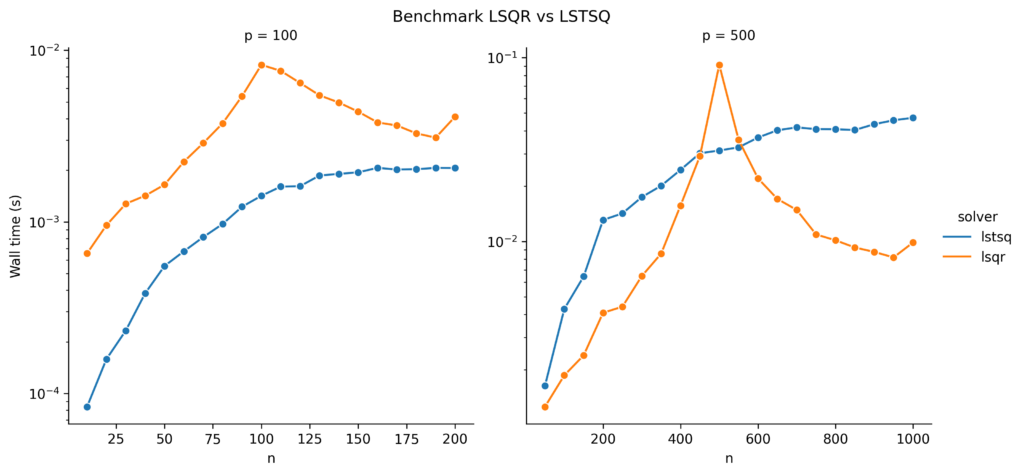

The left plot already looks a bit suspicious around n=p. But what is happening on the right side? Where does this spike of LSQR come from? And why does the standard least squares solver, SVD-based lstsq, not show this spike?

When I saw these results, I thought something might be wrong with LSQR and opened an issue on the scipy github repository, see https://github.com/scipy/scipy/issues/11204. The community there is really fantastic. Brett Naul pointed me to ….

The Marchenko–Pastur Distribution

The Marchenko–Pastur distribution is the distribution of the eigenvalues (singular values of square matrices) of certain random matrices in the large sample limit. Given a random matrix A \in \mathbb{R}^{n,p} with i.i.d. entries A_{ij} having zero mean, \mathbb{E}[A_{ij}] = 0, and finite variance, \mathrm{Var}[A_{ij}] = \sigma^2 < \infty, we define the matrix Y_n = \frac{1}{n}A^T A \in \mathbb{R}^{p,p}. As square and even symmetric matrix, Y_n has a simpler SVD, namely Y_n = V \Sigma V^T. One can in fact show that V is the same as in the SVD of A and that the diagonal matrix \Sigma = \frac{1}{n}S^TS contains the squared singular values of A and \min(0, p-n) extra zero values. The (diagonal) values of \Sigma are called eigenvalues \lambda_1, \ldots, \lambda_p of Y_n. Note/ that the eigenvalues are themselves random variables, and we are interested in their probability distribution or probability measure. We define the (random) measure \mu_p(B) = \frac{1}{p} \#\{\lambda_j \in B\} for all intervals B \subset \mathbb{R}.

The theorem of Marchenko and Pastur then states that for n, p \rightarrow \infty with \frac{p}{n} \rightarrow \rho , we have \mu_p \rightarrow \mu, where

\mu(B) = \begin{cases} (1-\frac{1}{\rho})\mathbb{1}_{0\in B} + \nu(B),\quad &\rho > 1 \\ \nu(B), \quad & 0\leq\rho\leq 1 \end{cases} \,,

\nu(x) = \frac{1}{2\pi\sigma^2} \frac{\sqrt{(\rho_+ - x)(x - \rho_-)}}{\rho x} \mathbb{1}_{x \in [\rho_-, \rho_+]} dx\,,

\rho_{\pm} = \sigma^2 (1\pm\sqrt{\rho})^2 \,.

We can at least derive the point mass at zero for \rho>1 \Leftrightarrow p>n: We said above that \Sigma contains p-n extra zeros and those correspond to a density of \frac{p-n}{p}=1 – \frac{1}{\rho} at zero.

A lot of math so far. Just note that the assumptions on A are exactly met by the one in our benchmark above. Also note that the normal equations can be expressed in terms of Y_n as n Y_n x = A^Tb.

Empirical Confirmation of the Marchenko–Pastur Distribution

Before we come back to the spikes in our benchmark, let us have a look and see how good the Marchenko–Pastur distribution is approximated for finite sample size. We choose n=1000, p=500 which gives \rho=\frac{1}{2}. We plot a histrogram of the eigenvalues next to the Marchenko–Pastur distribution.

def marchenko_pastur_mu(x, rho, sigma2=1):
    x = np.atleast_1d(x).astype(float)
    rho_p = sigma2 * (1 + np.sqrt(rho)) ** 2
    rho_m = sigma2 * (1 - np.sqrt(rho)) ** 2
    mu = np.zeros_like(x)
    is_nonzero = (rho_m < x) & (x < rho_p)
    x_valid = x[is_nonzero]
    factor = 1 / (2 * np.pi * sigma2 * rho)
    mu[is_nonzero] = factor / x_valid
    mu[is_nonzero] *= np.sqrt((rho_p - x_valid) * (x_valid - rho_m))
    if rho > 1:
        mu[x == 0] = 1 - 1 / rho
    return mu

fig, ax = plt.subplots()

n, p = 1000, 500
A = X.reshape(n, p)
Y = 1/n * A.T @ A
eigenvals, _ = np.linalg.eig(Y)
ax.hist(eigenvals.real, bins=50, density=True, label="histogram")
x = np.linspace(0, np.max(eigenvals.real), 100)
ax.plot(x, marchenko_pastur_mu(x, rho=p/n), label="MP distribution")
ax.legend()
ax.set_xlabel("eigenvalue")
ax.set_ylabel("probability")
ax.set_title("Empirical evidence for n=1000, p=500, rho=0.5")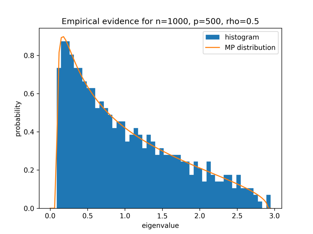

I have to say, I am very impressed by this good agreement for n=1000, which is far from being huge.

Conclusion

Let’s visualize the Marchenko–Pastur distribution Y_n for several ratios \rho and fix \sigma=1:

fig, ax = plt.subplots()

rho_list = [0.5, 1, 1.5]
x = np.linspace(0, 5, 1000)[1:] # exclude 0
for rho in rho_list:
    y = marchenko_pastur_mu(x, rho)
    line, = ax.plot(x, y, label=f"rho={rho}")
    # plot zero point mass
    if rho > 1:
        ax.scatter(0, marchenko_pastur_mu(0, rho), color = line.get_color())

ax.set_ylim(None, 1.2)
ax.legend()
ax.set_title("Marchenko-Pastur Distribution")
ax.set_xlabel("x")
ax.set_ylabel("dmu/dx")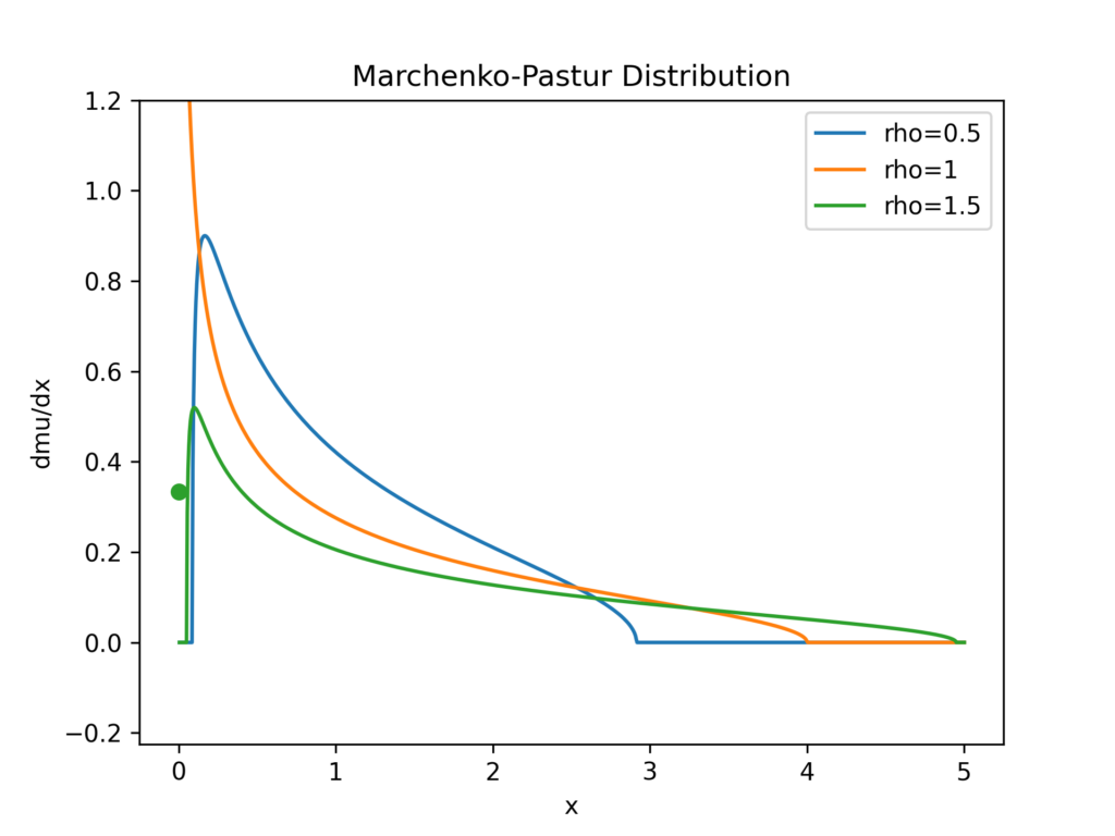

From this figure it becomes obvious that the closer the ratio \rho = 1, the higher the probability for very tiny eigenvalues. This results in a high probability for an ill-conditioned matrix A^TA coming from an ill-conditioned matrix A. Let’s confirm that:

p = 500
n_vec = []
c_vec = []
for n in np.arange(0.1, 2.05, 0.05):
    n = int(p*n)
    A = X[:n*p].reshape(n, p)
    n_vec.append(n)
    c_vec.append(np.linalg.cond(A))

fig, ax = plt.subplots()
ax.plot(n_vec, c_vec)
ax.set_xlabel("n")
ax.set_ylabel("condition number of A")
ax.set_title("Condition Number of A for p=500")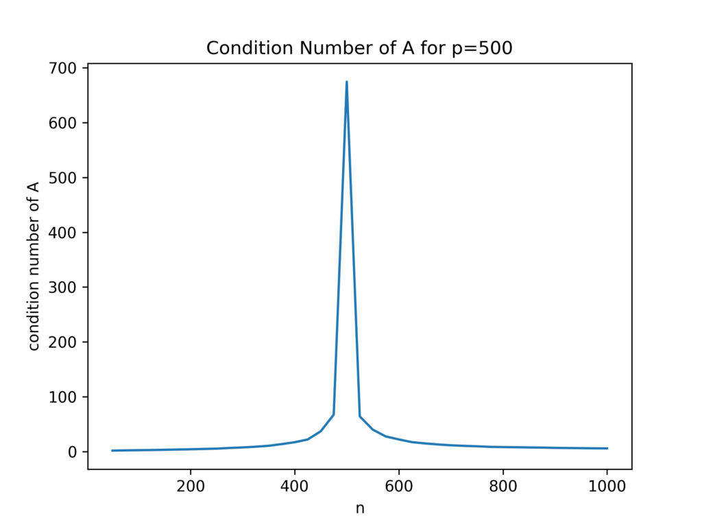

As a result of the ill-conditioned A, the LSQR solver has problems to achieve its tolerance criterion, needs more iterations, and takes longer time. This is exactly what we observed in the benchmark plots: the peak occurred around n=p. The SVD-based lstsq solver, on the other hand, does not use an iterative scheme and does not need more time for ill-conditioned matrices.

You find the accompanying notebook here: https://github.com/lorentzenchr/notebooks/blob/master/blogposts/2022-05-22%20from%20least%20squares%20benchmarks%20to%20the%20marchenko-pastur%20distribution.ipynb