Author: Christian Lorentzen

  • Feature Subsampling For Random Forest Regression

    TLDR: The number of subsampled features is a main source of randomness and an important parameter in random forests. Mind the different default values across implementations.

    Randomness in Random Forests

    Random forests are very popular machine learning models. They are build from easily understandable and well visualizable decision trees and give usually good predictive performance without the need for excessive hyperparameter tuning. Some drawbacks are that they do not scale well to very large datasets and that their predictions are discontinuous on continuous features.

    A key ingredient for random forests is—no surprise here—randomness. The two main sources for randomness are:

    • Feature subsampling in every node split when fitting decision trees.
    • Row subsampling (bagging) of the training dataset for each decision tree.

    In this post, we want to investigate the first source, feature subsampling, with a special focus on regression problems on continuous targets (as opposed to classification).

    Feature Subsampling

    In his seminal paper, Leo Breiman introduced random forests and pointed out several advantages of feature subsamling per node split. We cite from his paper:

    The forests studied here consist of using randomly selected inputs or combinations of inputs at each node to grow each tree. The resulting forests give accuracy that compare favorably with Adaboost. This class of procedures has desirable characteristics:

    i Its accuracy is as good as Adaboost and sometimes better.

    ii It’s relatively robust to outliers and noise.

    iii It’s faster than bagging or boosting.

    iv It gives useful internal estimates of error, strength, correlation and variable importance.

    v It’s simple and easily parallelized.

    Breiman, L. Random Forests. Machine Learning 45, 5–32 (2001).

    Note the focus on comparing with Adaboost at that time and the, in today’s view, relatively small datasets used for empirical studies in this paper.

    If the input data as p number of features (columns), implementations of random forests usually allow to specify how many features to consider at each split:

    ImplementationLanguageParameterDefault
    scikit-learn RandomForestRegressorPythonmax_featuresp
    scikit-learn RandomForestClassifierPythonmax_featuressqrt(p)
    rangerRmtrysqrt(p)
    randomForest regressionRmtryp/3
    randomForest classificationRmtrysqrt(p)
    H2O regressionPython & Rmtriesp/3
    H2O classificationPython & Rmtriessqrt(p)

    Note that the default of scikit-learn for regression is surprising because it switches of the randomness from feature subsampling rendering it equal to bagged trees!

    While empirical studies on the impact of feature for good default choices focus on classification problems, see the literature review in Probst et al 2019, we consider a set of regression problems with continuous targets. Note that different results might be more related to different feature spaces than to the difference between classification and regression.

    The hyperparameters mtry, sample size and node size are the parameters that control the randomness of the RF. […]. Out of these parameters, mtry is most influential both according to the literature and in our own experiments. The best value of mtry depends on the number of variables that are related to the outcome.

    Probst, P. et al. “Hyperparameters and tuning strategies for random forest.” Wiley Interdisciplinary Reviews: Data Mining and Knowledge Discovery 9 (2019): n. pag.

    Benchmarks

    We selected the following 13 datasets with regression problems:

    Datasetnumber of samplesnumber of used features p
    Allstate188,318130
    Bike_Sharing_Demand17,37912
    Brazilian_houses10’69212
    ames1’46079
    black_friday166’8219
    colleges7’06349
    delays_zurich_transport27’32717
    diamonds53’9406
    la_crimes1’468’82525
    medical_charges_nominal163’06511
    nyc-taxi-green-dec-2016581’83514
    particulate-matter-ukair-2017394’2999
    taxi581’83518

    Note that among those, there is no high dimensional dataset in the sense that p>number of samples.

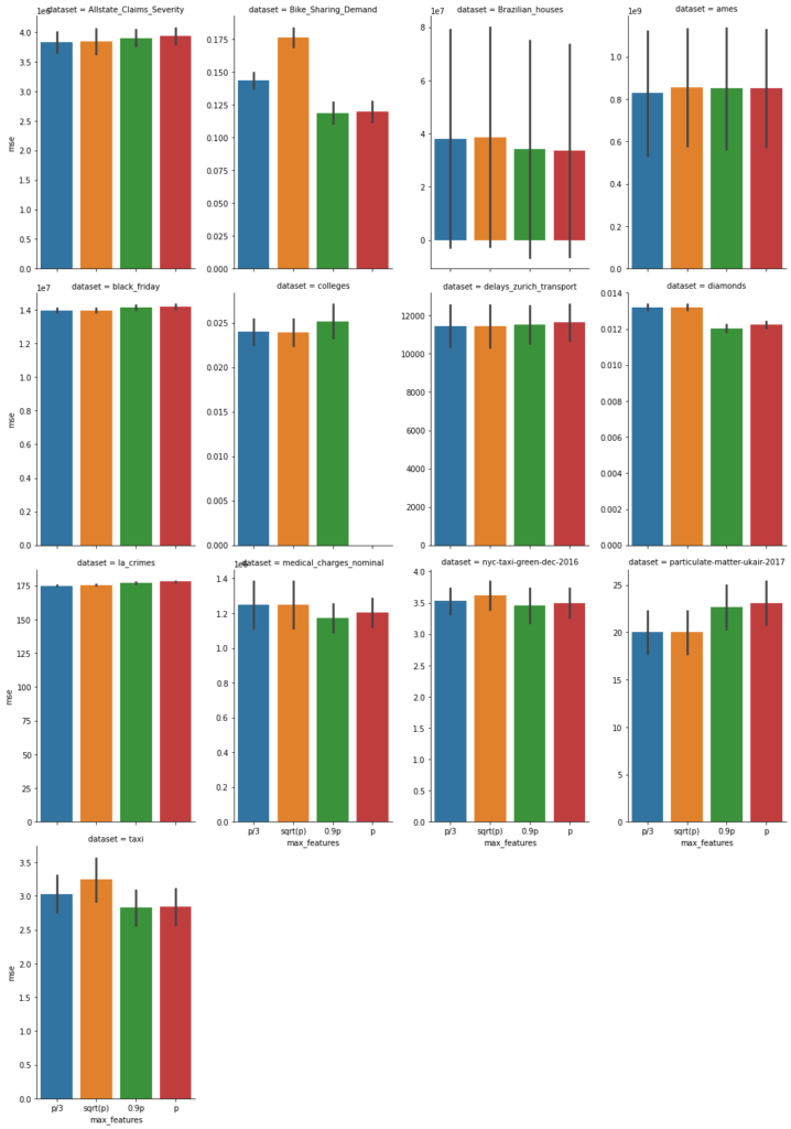
    On these, we fitted the scikit-learn (version 0.24) RandomForestRegressor (within a short pipeline handling missing values) with default parameters. We used 5-fold cross validation with 4 different values max_feature=p/3 (blue), sqrt(p) (orange), 0.9 p (green), and p (red). Now, we show the mean squared error with uncertainty bars (± one standard deviation of cross validation splits), the lower the better.

    In addition, we also report the fit time of each (5-fold) fit in seconds, again the lower the better.

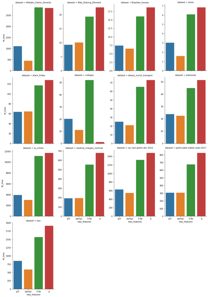
    Note that sqrt(p) is often smaller than p/3. With this in mind, this graphs show that fit time is about proportional to the number of features subsampled.

    Conclusion

    • The main tuning parameter of random forests is the number of features used for feature subsampling (max_features, mtry). Depending on the dataset, it has a relevant impact on the predictive performance.
    • The default of scikit-learn’s RandomForestRegressor seems odd. It produces bagged trees. This is a bit like using ridge regression with a zero penalty😉. However, it can be justified by our benchmarks above.

    The full code can be found here:

    https://github.com/lorentzenchr/notebooks/blob/master/blogposts/2021-08-19%20random_forests_max_features.ipynb

  • Least Squares Minimal Norm Solution

    Least squares is a cornerstone of linear algebra, optimization and therefore also for statistical and machine learning models. Given a matrix A ∈ Rn,p and a vector b ∈ Rn, we search for

    x^\star = \argmin_{x \in R^p} ||Ax - b||^2

    Translation for regression problems: Search for coefficients β→x given the design or features matrix X→A and target y→b.

    In the case of a singular matrix A or an underdetermined setting n<p, the above definition is not precise and permits many solutions x. In those cases, a more precise definition is the minimum norm solution of least squares:

    x^\star = \argmin_{x} ||x||^2
    \quad \text{subject to} \quad
    \min_{x \in R^p} ||Ax - b||^2

    In words: We solve the least squares problem and choose the solution with minimal Euclidean norm.

    We will show step by step what this means on a series on overdetermined systems. In linear regression with more observations than features, n>p, one says the system is overdetermined, leading to ||Ax^\star-b||^2 > 0 in most cases.

    Regular System

    Let’s start with a well-behaved example. To have good control over the matrix, we construct it by its singular value decomposition (SVD) A=USV’ with orthogonal matrices U and V and diagonal matrix S. Recall that S has only non-negative entries and — for regular matrices — even strictly positive values. Therefore, we start by setting \operatorname{diag}(S) = (1, 2, 3, 4, 5).

    from pprint import pprint
    import matplotlib.pyplot as plt
    import numpy as np
    from numpy.linalg import norm
    from scipy.stats import ortho_group
    from scipy import linalg
    from scipy.sparse import linalg as spla
    
    
    def generate_U_S_Vt(n=10, p=5, random_state=532):
        """Generate SVD to construct a regular matrix A.
        
        A has n rows, p columns.
        
        Returns
        -------
        U: orthogonal matrix
        S: diagonal matrix
        Vt: orthogonal matrix
        """
        r = min(n, p)
        S = np.diag(1.0 * np.arange(1, 1 + r))
        if n > p:
            # add rows with value 0
            S = np.concatenate((S, np.zeros((n - p, p))), axis=0)
        elif p > n:
            # add columns with value 0
            S = np.concatenate((S, np.zeros((n, p - n))), axis=1)
        U = ortho_group.rvs(n, random_state=random_state)
        Vt = ortho_group.rvs(p, random_state=random_state + 1)
        return U, S, Vt
    
    
    def solve_least_squares(A, b):
        """Solve least squares with several methods.
        
        Returns
        ------
        x : dictionary with solver and solution
        """
        x = {}
        x["gelsd"] = linalg.lstsq(A, b, lapack_driver="gelsd")[0]
        x["gelsy"] = linalg.lstsq(A, b, lapack_driver="gelsy")[0]
        x["lsqr"] = spla.lsqr(A, b)[0]
        x["lsmr"] = spla.lsmr(A, b)[0]
        x["normal_eq"] = linalg.solve(A.T @ A, A.T @ b, assume_a="sym")
    
        return x
    
    
    def print_dict(d):
        np.set_string_function(np.array2string)
        pprint(d)
        np.set_string_function(None)
    
    
    np.set_printoptions(precision=5)
    
    
    n = 10
    p = 5
    
    U, S, Vt = generate_U_S_Vt(n=n, p=p)
    A = U @ S @ Vt
    
    x_true = np.round(6 * Vt.T[:p, 0])  # interesting choice
    rng = np.random.default_rng(157)
    noise = rng.standard_normal(n)
    b = A @ x_true + noise
    
    S_inv = np.copy(S.T)
    S_inv[S_inv>0] = 1/S_inv[S_inv>0]
    
    x_exact = Vt.T @ S_inv @ U.T @ b
    
    print(f"x_exact = {x_exact}")
    print_dict(solve_least_squares(A, b))
    x_exact = [ 0.78087 -4.74942 -0.99938 -2.38327 -3.7431 ] {'gelsd': [ 0.78087 -4.74942 -0.99938 -2.38327 -3.7431 ],  'gelsy': [ 0.78087 -4.74942 -0.99938 -2.38327 -3.7431 ],  'lsmr': [ 0.78087 -4.74942 -0.99938 -2.38327 -3.7431 ],  'lsqr': [ 0.78087 -4.74942 -0.99938 -2.38327 -3.7431 ],  'normal_eq': [ 0.78087 -4.74942 -0.99938 -2.38327 -3.7431 ]}

    We see that all least squares solvers do well on regular systems, be it the LAPACK routines for direct least squares, GELSD and GELSY, the iterative solvers LSMR and LSQR or solving the normal equations by the LAPACK routine SYSV for symmetric matrices.

    Singular System

    We convert our regular matrix in a singular one by setting its first diagonal element to zero.

    S[0, 0] = 0
    A = U @ S @ Vt
    
    S_inv = np.copy(S.T)
    S_inv[S_inv>0] = 1/S_inv[S_inv>0]
    
    # Minimum Norm Solution
    x_exact = Vt.T @ S_inv @ U.T @ b
    
    print(f"x_exact = {x_exact}")
    x_solution = solve_least_squares(A, b)
    print_dict(x_solution)
    x_exact = [-0.21233  0.00708  0.34973 -0.30223 -0.0235 ] {'gelsd': [-0.21233  0.00708  0.34973 -0.30223 -0.0235 ],  'gelsy': [-0.21233  0.00708  0.34973 -0.30223 -0.0235 ],  'lsmr': [-0.21233  0.00708  0.34973 -0.30223 -0.0235 ],  'lsqr': [-0.21233  0.00708  0.34973 -0.30223 -0.0235 ],  'normal_eq': [-0.08393 -0.60784  0.17531 -0.57127 -0.50437]}

    As promised by their descriptions, the first four solvers find the minimum norm solution. If you run the code yourself, you will get a LinAlgWarning from the normal equation solver. The output confirms it: Solving normal equations for singular systems is a bad idea. However, a closer look reveals the following

    print(f"norm of x:\n"
          f"x_exact: {norm(x_exact)}\n"
          f"normal_eq: {norm(x_solution['normal_eq'])}\n"
         )
    print(f"norm of Ax-b:\n"
          f"x_exact: {norm(A @ x_exact - b)}\n"
          f"normal_eq: {norm(A @ x_solution['normal_eq'] - b)}"
         )
    norm of x:
    x_exact:   0.5092520023062155
    normal_eq: 0.993975690303498
    
    norm of Ax-b:
    x_exact:   6.9594032092014935
    normal_eq: 6.9594032092014935 

    Although the solution of the normal equations seems far off, it reaches the same minimum of the least squares problem and is thus a viable solution. Especially in iterative algorithms, the fact that the norm of the solution vector is large, at least larger than the minimum norm solution, is an undesirable property.

    Minimum Norm

    As the blogpost title advertises the minimum norm solution and a figure is still missing, we will visualize the many solutions to the least squares problem. But how to systematically construct different solutions? Luckily, we already have the SVD of A. The columns of V that multiply with the zero values of D, let’s call it V1, give us the null space of A, i.e. AV1 t = 0 for any vector t. In our example, there is only one such zero diagonal element, V1 is just one column and t reduces to a number.

    t = np.linspace(-3, 3, 100)  # free parameter
    # column vectos of x_lsq are least squares solutions
    x_lsq = (x_exact + Vt.T[:, 0] * t.reshape(-1, 1)).T
    x_norm = np.linalg.norm(x_lsq, axis=0)
    lsq_norm = np.linalg.norm(A @ x_lsq - b.reshape(-1, 1), axis=0)
    
    plt.plot(t, 2 * x_norm, label="2 * norm of x")
    plt.plot(t, lsq_norm, label="norm of Ax-b")
    plt.legend()
    plt.xlabel("t")
    plt.ylabel("Norm")
    plt.title("Euclidean norm of solution and residual")
    Norm of solution vector and residual of least squares

    In order to have both lines in one figure, we scaled the norm of the solution vector by a factor of two. We see that all vectors achieve the same objective, i.e. Euclidean norm of the residuals Ax – b, while t=0 has minimum norm among those solution vectors.

    Tiny Perturbation of b

    Let us also have a look what happens if we add a tiny perturbation to the vector b.

    eps = 1e-10
    print(f"x_exact = {x_exact}")
    print_dict(solve_least_squares(A, b + eps))
    x_exact = [-0.21233  0.00708  0.34973 -0.30223 -0.0235 ] {'gelsd': [-0.21233  0.00708  0.34973 -0.30223 -0.0235 ],  'gelsy': [-0.21233  0.00708  0.34973 -0.30223 -0.0235 ],  'lsmr': [-0.21233  0.00708  0.34973 -0.30223 -0.0235 ],  'lsqr': [-0.21233  0.00708  0.34973 -0.30223 -0.0235 ],  'normal_eq': [-0.12487 -0.41176  0.23093 -0.48548 -0.35104]}

    We see that the first four solvers are stable while the solving the normal equations shows large deviations compared to the unperturbed system above. For example, compare the first vector element of -0.21 vs -0.12 even for a perturbation as tiny as 1.0e-10.

    Ill-Conditioned System

    The last section showed an example of an ill-conditioned system. By ill-conditioned we mean a huge difference between largest and smallest eigenvalue of A, the ratio of which is called condition number. We can achieve this by setting the first diagonal element of S to a tiny positive number instead of exactly zero.

    S[0, 0] = 1e-10
    A = U @ S @ Vt
    
    S_inv = np.copy(S.T)
    S_inv[S_inv>0] = 1/S_inv[S_inv>0]
    
    # Minimum Norm Solution
    x_exact = Vt.T @ S_inv @ U.T @ b
    
    print(f"x_exact = {x_exact}")
    print_dict(solve_least_squares(A, b))
    x_exact = [ 9.93195e+09 -4.75650e+10 -1.34911e+10 -2.08104e+10 -3.71960e+10]
    {'gelsd': [ 9.93194e+09 -4.75650e+10 -1.34910e+10 -2.08104e+10 -3.71960e+10],
     'gelsy': [ 9.93196e+09 -4.75650e+10 -1.34911e+10 -2.08104e+10 -3.71961e+10],
     'lsmr': [-0.21233  0.00708  0.34973 -0.30223 -0.0235 ],
     'lsqr': [-0.21233  0.00708  0.34973 -0.30223 -0.0235 ],
     'normal_eq': [  48559.67679 -232557.57746  -65960.92822 -101747.66128 -181861.06429]}
    print(f"norm of x:\n"
          f"x_exact:   {norm(x_exact)}\n"
          f"lsqr:      {norm(x_solution['lsqr'])}\n"
          f"normal_eq: {norm(x_solution['normal_eq'])}\n"
         )
    print(f"norm of Ax-b:\n"
          f"x_exact:   {norm(A @ x_exact - b)}\n"
          f"lsqr:      {norm(A @ x_solution['lsqr'] - b)}\n"
          f"normal_eq: {norm(A @ x_solution['normal_eq'] - b)}"
         )
    norm of x:
    x_exact:   66028022639.34349
    lsqr:      0.5092520023062157
    normal_eq: 0.993975690303498
    
    norm of Ax-b:
    x_exact:   2.1991587442017146
    lsqr:      6.959403209201494
    normal_eq: 6.959403209120507

    Several points are interesting to observe:

    • The exact solution has a very large norm. A tiny change in the matrix A compared to the singular system changed the solution dramatically!
    • Normal equation and iterative solvers LSQR and LSMR fail badly and don’t find the solution with minimal residual. All three seem to find solutions with the same norm as the singular system from above.
    • The iterative solvers indeed find exactly the same solutions as for the singular system.

    Note, that LSQR and LSMR can be fixed by requiring a higher accuracy via the parameters atol and btol.

    Wrap-Up

    Solving least squares problems is fundamental for many applications. While regular systems are more or less easy to solve, singular as well as ill-conditioned systems have intricacies: Multiple solutions and sensibility to small perturbations. At least, the minimum norm solution always gives a well defined unique answer and direct solvers find it reliably.

    The Python notebook can be found in the usual github repository: 2021-05-02 least_squares_minimum_norm_solution.ipynb

    References

    Very good, concise reference:

    Good source with respect to Ordinary Least Squares (OLS)

    • Trevor Hastie, Andrea Montanari, Saharon Rosset, Ryan J. Tibshirani, Surprises in High-Dimensional Ridgeless Least Squares Interpolation
      https://arxiv.org/abs/1903.08560
  • Swiss Mortality

    Lost in Translation between R and Python 3

    Hello again!

    This is the third article in our series “Lost in Translation between R and Python”. The aim of this series is to provide high-quality R and Python 3 code to achieve some non-trivial tasks. If you are to learn R, check out the R tab below. Similarly, if you are to learn Python, the Python tab will be your friend.

    Post 2: https://lorentzen.ch/index.php/2021/01/26/covid-19-deaths-per-mio/

    Before diving into the data analysis, I would like to share with you that writing this text brought back some memories from my first year as an actuary. Indeed, I started in life insurance and soon switched to non-life. While investigating mortality may be seen as a dry matter, it reveals some interesting statistical problems which have to be properly addressed before drawing conclusions.

    Similar to Post 2, we use a publicly available data, this time from the Human Mortality Database and from the Federal Statistical Office of Switzerland, in order to calculate crude death rates, i.e. number of deaths per person alive per year. This time, we look at a longer time periode of 20 and over 100 years and take all causes of death into account. We caution against any misinterpretation: We show only crude death rates (CDR) which do not take into account any demographic shifts like changing distributions of age or effects from measures taken against COVID-19.

    Let us start with producing the first figure. We fetch the data from the internet, pick some countries of interest, focus on males and females combined only, aggregate and plot. The Python version uses the visualization library altair, which can generate interactive charts. Unfortunately, we can only show a static version in the blog post. If someone knows how to render Vega-Light charts in wordpress, I’d be very interested in a secure solution.

    library(tidyverse)
    library(lubridate)
    
    # Fetch data
    df_original = read_csv(
      "https://www.mortality.org/Public/STMF/Outputs/stmf.csv",
      skip = 2
    )
    
    # 1. Select countries of interest and only "both" sexes
    # Note: Germany "DEUTNP" and "USA" have short time series
    # 2. Change to ISO-3166-1 ALPHA-3 codes
    # 3.Create population pro rata temporis (exposure) to ease aggregation
    df_mortality <- df_original %>% 
      filter(CountryCode %in% c("CAN", "CHE", "FRATNP", "GBRTENW", "SWE"),
             Sex == "b") %>% 
      mutate(CountryCode = recode(CountryCode, "FRATNP" = "FRA",
                                  "GBRTENW" = "England & Wales"),
             population = DTotal / RTotal,
             Year = ymd(Year, truncated = 2))
    
    # Data aggregation per year and country
    df <- df_mortality %>%
      group_by(Year, CountryCode) %>% 
      summarise(CDR = sum(DTotal) / sum(population), 
                .groups = "drop")
    
    ggplot(df, aes(x = Year, y = CDR, color = CountryCode)) +
      geom_line(size = 1) +
      ylab("Crude Death Rate per Year") +
      theme(legend.position = c(0.2, 0.8))
    import pandas as pd
    import altair as alt
    
    
    # Fetch data
    df_mortality = pd.read_csv(
        "https://www.mortality.org/Public/STMF/Outputs/stmf.csv",
        skiprows=2,
    )
    
    # Select countdf_mortalityf interest and only "both" sexes
    # Note: Germany "DEUTNP" and "USA" have short time series
    df_mortality = df_mortality[
        df_mortality["CountryCode"].isin(["CAN", "CHE", "FRATNP", "GBRTENW", "SWE"])
        & (df_mortality["Sex"] == "b")
    ].copy()
    
    # Change to ISO-3166-1 ALPHA-3 codes
    df_mortality["CountryCode"].replace(
        {"FRATNP": "FRA", "GBRTENW": "England & Wales"}, inplace=True
    )
    
    # Create population pro rata temporis (exposure) to ease aggregation
    df_mortality = df_mortality.assign(
        population=lambda df: df["DTotal"] / df["RTotal"]
    )
    
    # Data aggregation per year and country
    df_mortality = (
        df_mortality.groupby(["Year", "CountryCode"])[["population", "DTotal"]]
        .sum()
        .assign(CDR=lambda x: x["DTotal"] / x["population"])
        # .filter(items=["CDR"])  # make df even smaller
        .reset_index()
        .assign(Year=lambda x: pd.to_datetime(x["Year"], format="%Y"))
    )
    
    chart = (
        alt.Chart(df_mortality)
        .mark_line()
        .encode(
            x="Year:T",
            y=alt.Y("CDR:Q", scale=alt.Scale(zero=False)),
            color="CountryCode:N",
        )
        .properties(title="Crude Death Rate per Year")
        .interactive()
    )
    # chart.save("crude_death_rate.html")
    chart
    Crude death rate (CDR) for Canada (CAN), Switzerland (CHE), England & Wales, France (FRA) and Sweden (SWE). Data as of 07.02.2021.

    Note that the y-axis does not start at zero. Nevertheless, we see values between 0.007 and 0.014, which is twice as large. While 2020 shows a clear raise in mortality, for some countries more dramatic than for others, the values of 2021 are still preliminary. For 2021, the data is still incomplete and the yearly CDR is based on a small observation period and hence on a smaller population pro rata temporis. On top, there might be effects from seasonality. To sum up, it means that there is a larger uncertainty for 2021 than for previous whole years.

    For Switzerland, it is also possible to collect data for over 100 years. As the code for data fetching and preparation becomes a bit lengthy, we won’t bother you with it. You can find it in the notebooks linked below. Note that we added the value of 2020 from the figure above. This seems legit as the CDR of both data sources agree within less than 1% relative error.

    Crude death rate (CDR) for Switzerland from 1901 to 2020.

    Again, note that the left y-axis does not start at zero, but the right y-axis does. One can see several interesting facts:

    • The Swiss population is and always was growing for the last 120 years—with the only exception around 1976.
    • The Spanish flu between 1918 and 1920 caused by far the largest peak in mortality in the last 120 years.
    • The second world war is not visible in the mortality in Switzerland.
    • Overall, the mortality is decreasing.

    The Python notebook and R code can be found at: