Least squares is a cornerstone of linear algebra, optimization and therefore also for statistical and machine learning models. Given a matrix A ∈ Rn,p and a vector b ∈ Rn, we search for
x^\star = \argmin_{x \in R^p} ||Ax - b||^2Translation for regression problems: Search for coefficients β→x given the design or features matrix X→A and target y→b.
In the case of a singular matrix A or an underdetermined setting n<p, the above definition is not precise and permits many solutions x⋆. In those cases, a more precise definition is the minimum norm solution of least squares:
x^\star = \argmin_{x} ||x||^2
\quad \text{subject to} \quad
\min_{x \in R^p} ||Ax - b||^2
In words: We solve the least squares problem and choose the solution with minimal Euclidean norm.
We will show step by step what this means on a series on overdetermined systems. In linear regression with more observations than features, n>p, one says the system is overdetermined, leading to ||Ax^\star-b||^2 > 0
Regular System
Let’s start with a well-behaved example. To have good control over the matrix, we construct it by its singular value decomposition (SVD) A=USV’ with orthogonal matrices U and V and diagonal matrix S. Recall that S has only non-negative entries and — for regular matrices — even strictly positive values. Therefore, we start by setting \operatorname{diag}(S) = (1, 2, 3, 4, 5)
from pprint import pprint
import matplotlib.pyplot as plt
import numpy as np
from numpy.linalg import norm
from scipy.stats import ortho_group
from scipy import linalg
from scipy.sparse import linalg as spla


def generate_U_S_Vt(n=10, p=5, random_state=532):
    """Generate SVD to construct a regular matrix A.

    A has n rows, p columns.

    Returns
    -------
    U: orthogonal matrix
    S: diagonal matrix
    Vt: orthogonal matrix
    """
    r = min(n, p)
    S = np.diag(1.0 * np.arange(1, 1 + r))
    if n > p:
        # add rows with value 0
        S = np.concatenate((S, np.zeros((n - p, p))), axis=0)
    elif p > n:
        # add columns with value 0
        S = np.concatenate((S, np.zeros((n, p - n))), axis=1)
    U = ortho_group.rvs(n, random_state=random_state)
    Vt = ortho_group.rvs(p, random_state=random_state + 1)
    return U, S, Vt


def solve_least_squares(A, b):
    """Solve least squares with several methods.

    Returns
    ------
    x : dictionary with solver and solution
    """
    x = {}
    x["gelsd"] = linalg.lstsq(A, b, lapack_driver="gelsd")[0]
    x["gelsy"] = linalg.lstsq(A, b, lapack_driver="gelsy")[0]
    x["lsqr"] = spla.lsqr(A, b)[0]
    x["lsmr"] = spla.lsmr(A, b)[0]
    x["normal_eq"] = linalg.solve(A.T @ A, A.T @ b, assume_a="sym")

    return x


def print_dict(d):
    np.set_string_function(np.array2string)
    pprint(d)
    np.set_string_function(None)


np.set_printoptions(precision=5)


n = 10
p = 5

U, S, Vt = generate_U_S_Vt(n=n, p=p)
A = U @ S @ Vt

x_true = np.round(6 * Vt.T[:p, 0])  # interesting choice
rng = np.random.default_rng(157)
noise = rng.standard_normal(n)
b = A @ x_true + noise

S_inv = np.copy(S.T)
S_inv[S_inv>0] = 1/S_inv[S_inv>0]

x_exact = Vt.T @ S_inv @ U.T @ b

print(f"x_exact = {x_exact}")
print_dict(solve_least_squares(A, b))
x_exact = [ 0.78087 -4.74942 -0.99938 -2.38327 -3.7431 ] {'gelsd': [ 0.78087 -4.74942 -0.99938 -2.38327 -3.7431 ], 'gelsy': [ 0.78087 -4.74942 -0.99938 -2.38327 -3.7431 ], 'lsmr': [ 0.78087 -4.74942 -0.99938 -2.38327 -3.7431 ], 'lsqr': [ 0.78087 -4.74942 -0.99938 -2.38327 -3.7431 ], 'normal_eq': [ 0.78087 -4.74942 -0.99938 -2.38327 -3.7431 ]}We see that all least squares solvers do well on regular systems, be it the LAPACK routines for direct least squares, GELSD and GELSY, the iterative solvers LSMR and LSQR or solving the normal equations by the LAPACK routine SYSV for symmetric matrices.
Singular System
We convert our regular matrix in a singular one by setting its first diagonal element to zero.
S[0, 0] = 0
A = U @ S @ Vt

S_inv = np.copy(S.T)
S_inv[S_inv>0] = 1/S_inv[S_inv>0]

# Minimum Norm Solution
x_exact = Vt.T @ S_inv @ U.T @ b

print(f"x_exact = {x_exact}")
x_solution = solve_least_squares(A, b)
print_dict(x_solution)
x_exact = [-0.21233 0.00708 0.34973 -0.30223 -0.0235 ] {'gelsd': [-0.21233 0.00708 0.34973 -0.30223 -0.0235 ], 'gelsy': [-0.21233 0.00708 0.34973 -0.30223 -0.0235 ], 'lsmr': [-0.21233 0.00708 0.34973 -0.30223 -0.0235 ], 'lsqr': [-0.21233 0.00708 0.34973 -0.30223 -0.0235 ], 'normal_eq': [-0.08393 -0.60784 0.17531 -0.57127 -0.50437]}As promised by their descriptions, the first four solvers find the minimum norm solution. If you run the code yourself, you will get a LinAlgWarning from the normal equation solver. The output confirms it: Solving normal equations for singular systems is a bad idea. However, a closer look reveals the following
print(f"norm of x:\n"
      f"x_exact: {norm(x_exact)}\n"
      f"normal_eq: {norm(x_solution['normal_eq'])}\n"
     )
print(f"norm of Ax-b:\n"
      f"x_exact: {norm(A @ x_exact - b)}\n"
      f"normal_eq: {norm(A @ x_solution['normal_eq'] - b)}"
     )
norm of x:
x_exact: 0.5092520023062155
normal_eq: 0.993975690303498
norm of Ax-b:
x_exact: 6.9594032092014935
normal_eq: 6.9594032092014935 Although the solution of the normal equations seems far off, it reaches the same minimum of the least squares problem and is thus a viable solution. Especially in iterative algorithms, the fact that the norm of the solution vector is large, at least larger than the minimum norm solution, is an undesirable property.
Minimum Norm
As the blogpost title advertises the minimum norm solution and a figure is still missing, we will visualize the many solutions to the least squares problem. But how to systematically construct different solutions? Luckily, we already have the SVD of A. The columns of V that multiply with the zero values of D, let’s call it V1, give us the null space of A, i.e. AV1 t = 0 for any vector t. In our example, there is only one such zero diagonal element, V1 is just one column and t reduces to a number.
t = np.linspace(-3, 3, 100)  # free parameter
# column vectos of x_lsq are least squares solutions
x_lsq = (x_exact + Vt.T[:, 0] * t.reshape(-1, 1)).T
x_norm = np.linalg.norm(x_lsq, axis=0)
lsq_norm = np.linalg.norm(A @ x_lsq - b.reshape(-1, 1), axis=0)

plt.plot(t, 2 * x_norm, label="2 * norm of x")
plt.plot(t, lsq_norm, label="norm of Ax-b")
plt.legend()
plt.xlabel("t")
plt.ylabel("Norm")
plt.title("Euclidean norm of solution and residual")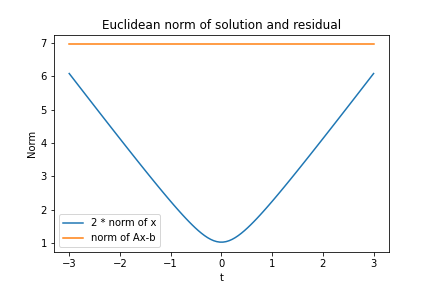
In order to have both lines in one figure, we scaled the norm of the solution vector by a factor of two. We see that all vectors achieve the same objective, i.e. Euclidean norm of the residuals Ax – b, while t=0 has minimum norm among those solution vectors.
Tiny Perturbation of b
Let us also have a look what happens if we add a tiny perturbation to the vector b.
eps = 1e-10
print(f"x_exact = {x_exact}")
print_dict(solve_least_squares(A, b + eps))
x_exact = [-0.21233 0.00708 0.34973 -0.30223 -0.0235 ] {'gelsd': [-0.21233 0.00708 0.34973 -0.30223 -0.0235 ], 'gelsy': [-0.21233 0.00708 0.34973 -0.30223 -0.0235 ], 'lsmr': [-0.21233 0.00708 0.34973 -0.30223 -0.0235 ], 'lsqr': [-0.21233 0.00708 0.34973 -0.30223 -0.0235 ], 'normal_eq': [-0.12487 -0.41176 0.23093 -0.48548 -0.35104]}We see that the first four solvers are stable while the solving the normal equations shows large deviations compared to the unperturbed system above. For example, compare the first vector element of -0.21 vs -0.12 even for a perturbation as tiny as 1.0e-10.
Ill-Conditioned System
The last section showed an example of an ill-conditioned system. By ill-conditioned we mean a huge difference between largest and smallest eigenvalue of A, the ratio of which is called condition number. We can achieve this by setting the first diagonal element of S to a tiny positive number instead of exactly zero.
S[0, 0] = 1e-10
A = U @ S @ Vt

S_inv = np.copy(S.T)
S_inv[S_inv>0] = 1/S_inv[S_inv>0]

# Minimum Norm Solution
x_exact = Vt.T @ S_inv @ U.T @ b

print(f"x_exact = {x_exact}")
print_dict(solve_least_squares(A, b))
x_exact = [ 9.93195e+09 -4.75650e+10 -1.34911e+10 -2.08104e+10 -3.71960e+10]
{'gelsd': [ 9.93194e+09 -4.75650e+10 -1.34910e+10 -2.08104e+10 -3.71960e+10],
'gelsy': [ 9.93196e+09 -4.75650e+10 -1.34911e+10 -2.08104e+10 -3.71961e+10],
'lsmr': [-0.21233 0.00708 0.34973 -0.30223 -0.0235 ],
'lsqr': [-0.21233 0.00708 0.34973 -0.30223 -0.0235 ],
'normal_eq': [ 48559.67679 -232557.57746 -65960.92822 -101747.66128 -181861.06429]}print(f"norm of x:\n"
f"x_exact: {norm(x_exact)}\n"
f"lsqr: {norm(x_solution['lsqr'])}\n"
f"normal_eq: {norm(x_solution['normal_eq'])}\n"
)
print(f"norm of Ax-b:\n"
f"x_exact: {norm(A @ x_exact - b)}\n"
f"lsqr: {norm(A @ x_solution['lsqr'] - b)}\n"
f"normal_eq: {norm(A @ x_solution['normal_eq'] - b)}"
)norm of x:
x_exact: 66028022639.34349
lsqr: 0.5092520023062157
normal_eq: 0.993975690303498
norm of Ax-b:
x_exact: 2.1991587442017146
lsqr: 6.959403209201494
normal_eq: 6.959403209120507Several points are interesting to observe:
- The exact solution has a very large norm. A tiny change in the matrix A compared to the singular system changed the solution dramatically!
- Normal equation and iterative solvers LSQR and LSMR fail badly and don’t find the solution with minimal residual. All three seem to find solutions with the same norm as the singular system from above.
- The iterative solvers indeed find exactly the same solutions as for the singular system.
Note, that LSQR and LSMR can be fixed by requiring a higher accuracy via the parameters atol and btol.
Wrap-Up
Solving least squares problems is fundamental for many applications. While regular systems are more or less easy to solve, singular as well as ill-conditioned systems have intricacies: Multiple solutions and sensibility to small perturbations. At least, the minimum norm solution always gives a well defined unique answer and direct solvers find it reliably.
The Python notebook can be found in the usual github repository: 2021-05-02 least_squares_minimum_norm_solution.ipynb
References
Very good, concise reference:
- Do Q Lee (2012), Numerically Efficient Methods For Solving Least Squares Problems
http://math.uchicago.edu/~may/REU2012/REUPapers/Lee.pdf
Good source with respect to Ordinary Least Squares (OLS)
- Trevor Hastie, Andrea Montanari, Saharon Rosset, Ryan J. Tibshirani, Surprises in High-Dimensional Ridgeless Least Squares Interpolation
https://arxiv.org/abs/1903.08560