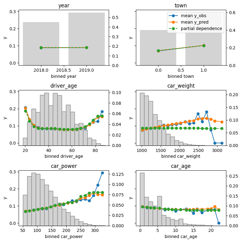
Christian and me did some code magic: Highly effective plots that help to build and inspect any model:
- Python: https://github.com/lorentzenchr/model-diagnostics
pip install model-diagnostics - R: https://github.com/mayer79/effectplots
install.packages("effectplots")
The functionality is best described by its output:


The plots show different types of feature effects relevant in modeling:
- Average observed: Descriptive effect (also interesting without model).
- Average predicted: Combined effect of all features. Also called “M Plot” (Apley 2020).
- Partial dependence: Effect of one feature, keeping other feature values constant (Friedman 2001).
- Number of observations or sum of case weights: Feature value distribution.
- R only: Accumulated local effects, an alternative to partial dependence (Apley 2020).
Both implementations…
- are highly efficient thanks to {Polars} in Python and {collapse} in R, and work on datasets with millions of observations,
- support case weights with all their statistics, ideal in insurance applications,
- calculate average residuals (not shown in the plots above),
- provide standard deviations/errors of average observed and bias,
- allow to switch to Plotly for interactive plots, and
- are highly customizable (the R package, e.g., allows to collapse rare levels after calculating statistics via the
update()method or to sort the features according to main effect importance).
In the spirit of our “Lost In Translation” series, we provide both high-quality Python and R code. We will use the same data and models as in one of our latest posts on how to build strong GLMs via ML + XAI.
Example
Let’s build a Poisson LightGBM model to explain the claim frequency given six traditional features in a pricing dataset on motor liability claims. 80% of the 1 Mio rows are used for training, the other 20% for evaluation. Hyper-parameters have been slightly tuned (not shown).
library(OpenML)
library(lightgbm)

dim(df <- getOMLDataSet(data.id = 45106L)$data)  # 1000000 7
head(df)

#   year town driver_age car_weight car_power car_age claim_nb
# 0 2018    1         51       1760       173       3        0
# 1 2019    1         41       1760       248       2        0
# 2 2018    1         25       1240       111       2        0
# 3 2019    0         40       1010        83       9        0
# 4 2018    0         43       2180       169       5        0
# 5 2018    1         45       1170       149       1        1

yvar <- "claim_nb"
xvars <- setdiff(colnames(df), yvar)

ix <- 1:800000
train <- df[ix, ]
test <- df[-ix, ]
X_train <- data.matrix(train[xvars])
X_test <- data.matrix(test[xvars])

# Training, using slightly optimized parameters found via cross-validation
params <- list(
  learning_rate = 0.05,
  objective = "poisson",
  num_leaves = 7,
  min_data_in_leaf = 50,
  min_sum_hessian_in_leaf = 0.001,
  colsample_bynode = 0.8,
  bagging_fraction = 0.8,
  lambda_l1 = 3,
  lambda_l2 = 5,
  num_threads = 7
)

set.seed(1)

fit <- lgb.train(
  params = params,
  data = lgb.Dataset(X_train, label = train$claim_nb),
  nrounds = 300
)
import matplotlib.pyplot as plt
from lightgbm import LGBMRegressor
from sklearn.datasets import fetch_openml

df = fetch_openml(data_id=45106, parser="pandas").frame
df.head()

#   year town driver_age car_weight car_power car_age claim_nb
# 0 2018    1         51       1760       173       3        0
# 1 2019    1         41       1760       248       2        0
# 2 2018    1         25       1240       111       2        0
# 3 2019    0         40       1010        83       9        0
# 4 2018    0         43       2180       169       5        0
# 5 2018    1         45       1170       149       1        1

# Train model on 80% of the data
y = df.pop("claim_nb")
n_train = 800_000
X_train, y_train = df.iloc[:n_train], y.iloc[:n_train]
X_test, y_test = df.iloc[n_train:], y.iloc[n_train:]

params = {
    "learning_rate": 0.05,
    "objective": "poisson",
    "num_leaves": 7,
    "min_child_samples": 50,
    "min_child_weight": 0.001,
    "colsample_bynode": 0.8,
    "subsample": 0.8,
    "reg_alpha": 3,
    "reg_lambda": 5,
    "verbose": -1,
}

model = LGBMRegressor(n_estimators=300, **params, random_state=1)
model.fit(X_train, y_train)
Let’s inspect the (main effects) of the model on the test data.
library(effectplots)

# 0.3 s
feature_effects(fit, v = xvars, data = X_test, y = test$claim_nb) |>
  plot(share_y = "all")
from model_diagnostics.calibration import plot_marginal

fig, axes = plt.subplots(3, 2, figsize=(8, 8), sharey=True, layout="tight")

# 2.3 s
for i, (feat, ax) in enumerate(zip(X_test.columns, axes.flatten())):
    plot_marginal(
        y_obs=y_test,
        y_pred=model.predict(X_test),
        X=X_test,
        feature_name=feat,
        predict_function=model.predict,
        ax=ax,
    )
    ax.set_title(feat)
    if i != 1:
        ax.legend().remove()
The output can be seen at the beginning of this blog post.
Here some model insights:
- Average predictions closely match observed frequencies. No clear bias is visible.
- Partial dependence shows that the year and the car weight almost have no impact (regarding their main effects), while the
driver_ageandcar_powereffects seem strongest. The shared y axes help to assess these. - Except for
car_weight, the partial dependence curve closely follows the average predictions. This means that the model effect seems to really come from the feature on the x axis, and not of some correlated other feature (as, e.g., withcar_weightwhich is actually strongly correlated withcar_power).
Final words
- Inspecting models has become much relaxed with above functions.
- The packages used offer much more functionality. Try them out! Or we will show them in later posts ;).
References
- Apley, Daniel W., and Jingyu Zhu. 2020. Visualizing the Effects of Predictor Variables in Black Box Supervised Learning Models. Journal of the Royal Statistical Society Series B: Statistical Methodology, 82 (4): 1059–1086. doi:10.1111/rssb.12377.
- Friedman, Jerome H. 2001. Greedy Function Approximation: A Gradient Boosting Machine. Annals of Statistics 29 (5): 1189–1232. doi:10.1214/aos/1013203451.
Leave a Reply