Interactions – where are you? – Michael's and Christian's Blog

This question sends shivers down the poor modelers spine…

The {hstats} R package introduced in our last post measures their strength using Friedman’s H-statistics, a collection of statistics based on partial dependence functions.

On Github, the preview version of {hstats} 1.0.0 out – I will try to bring it to CRAN in about one week (October 2023). Until then, try it via devtools::install_github("mayer79/hstats")

The current version offers:

H statistics per feature, feature pair, and feature triple
Multivariate predictions at no additional cost
A convenient API
Other important tools from explainable ML:
- performance calculations
- permutation importance (e.g., to select features for calculating H-statistics)
- partial dependence plots (including grouping, multivariate, multivariable)
- individual conditional expectations (ICE)
Case-weights are available for all methods, which is important, e.g., in insurance applications
The option for fast quantile approximation of H-statistics

This post has two parts:

Example with house-prices and XGBoost
Naive benchmark against {iml}, {DALEX}, and my old {flashlight}.

1. Example

Let’s model logarithmic sales prices of houses sold in Miami Dade County, a dataset prepared by Prof. Dr. Steven Bourassa, and available in {shapviz}. We use XGBoost with interaction constraints to provide a model additive in all structure information, but allowing for interactions between latitude/longitude for a flexible representation of geographic effects.

The following code prepares the data, splits the data into train and validation, and then fits an XGBoost model.

library(hstats)
library(shapviz)
library(xgboost)
library(ggplot2)

# Data preparation
colnames(miami) <- tolower(colnames(miami))
miami <- transform(miami, log_price = log(sale_prc))
x <- c("tot_lvg_area", "lnd_sqfoot", "latitude", "longitude",
       "structure_quality", "age", "month_sold")
coord <- c("longitude", "latitude")

# Modeling
set.seed(1)
ix <- sample(nrow(miami), 0.8 * nrow(miami))
train <- data.frame(miami[ix, ])
valid <- data.frame(miami[-ix, ])
y_train <- train$log_price
y_valid <- valid$log_price
X_train <- data.matrix(train[x])
X_valid <- data.matrix(valid[x])

dtrain <- xgb.DMatrix(X_train, label = y_train)
dvalid <- xgb.DMatrix(X_valid, label = y_valid)

ic <- c(
  list(which(x %in% coord) - 1),
  as.list(which(!x %in% coord) - 1)
)

# Fit via early stopping
fit <- xgb.train(
  params = list(
    learning_rate = 0.15, 
    objective = "reg:squarederror", 
    max_depth = 5,
    interaction_constraints = ic
  ),
  data = dtrain,
  watchlist = list(valid = dvalid),
  early_stopping_rounds = 20,
  nrounds = 1000,
  callbacks = list(cb.print.evaluation(period = 100))
)

Now it is time for a compact analysis with {hstats} to interpret the model:

average_loss(fit, X = X_valid, y = y_valid)  # 0.0247 MSE -> 0.157 RMSE

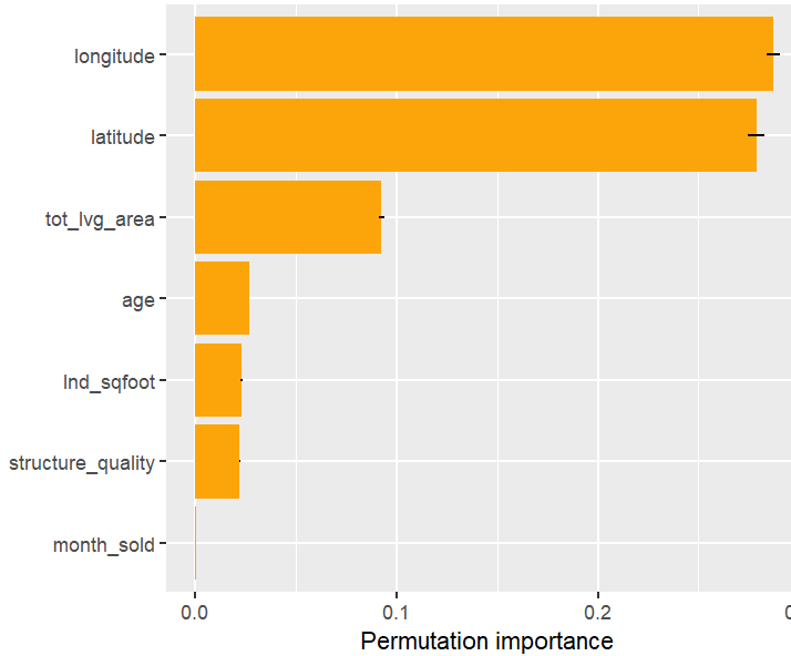
perm_importance(fit, X = X_valid, y = y_valid) |> 
  plot()

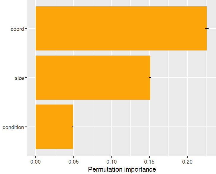
# Or combining some features
v_groups <- list(
  coord = c("longitude", "latitude"),
  size = c("lnd_sqfoot", "tot_lvg_area"),
  condition = c("age", "structure_quality")
)
perm_importance(fit, v = v_groups, X = X_valid, y = y_valid) |> 
  plot()

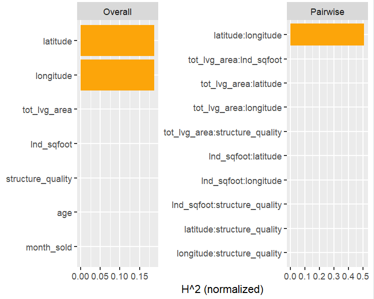
H <- hstats(fit, v = x, X = X_valid)
H
plot(H)
plot(H, zero = FALSE)
h2_pairwise(H, zero = FALSE, squared = FALSE, normalize = FALSE)
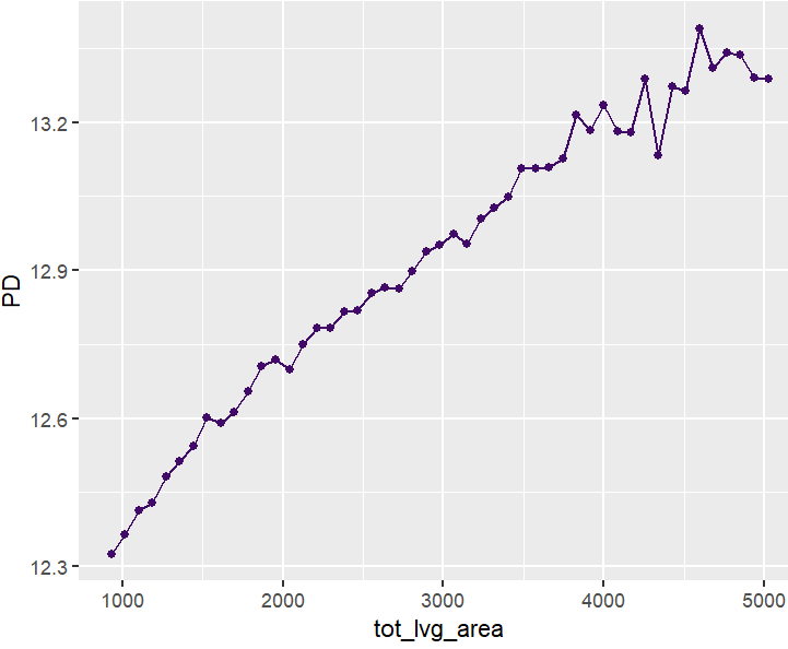
partial_dep(fit, v = "tot_lvg_area", X = X_valid) |> 
  plot()
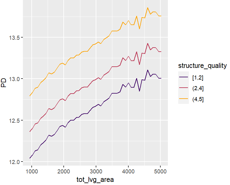
partial_dep(fit, v = "tot_lvg_area", X = X_valid, BY = "structure_quality") |> 
  plot(show_points = FALSE)
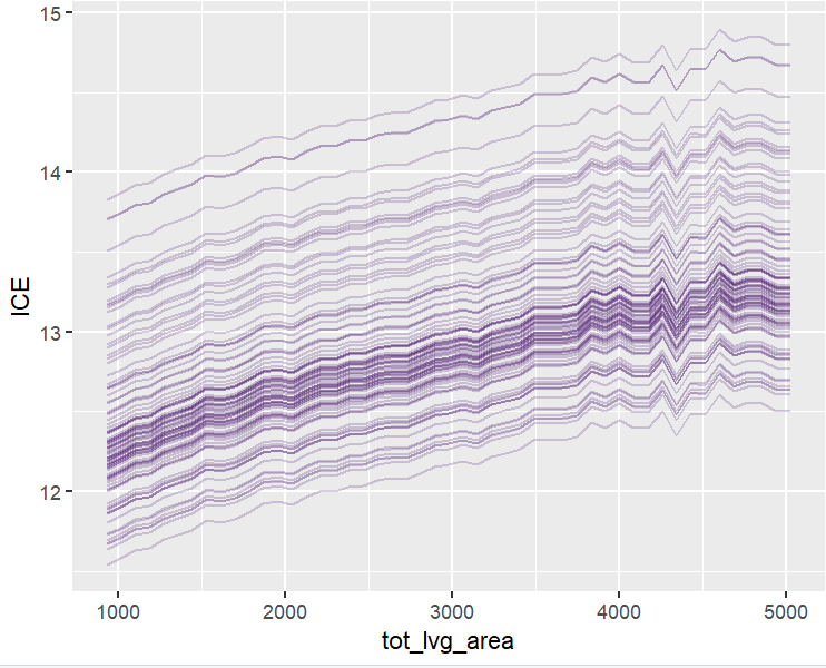
plot(ii <- ice(fit, v = "tot_lvg_area", X = X_valid))
plot(ii, center = TRUE)

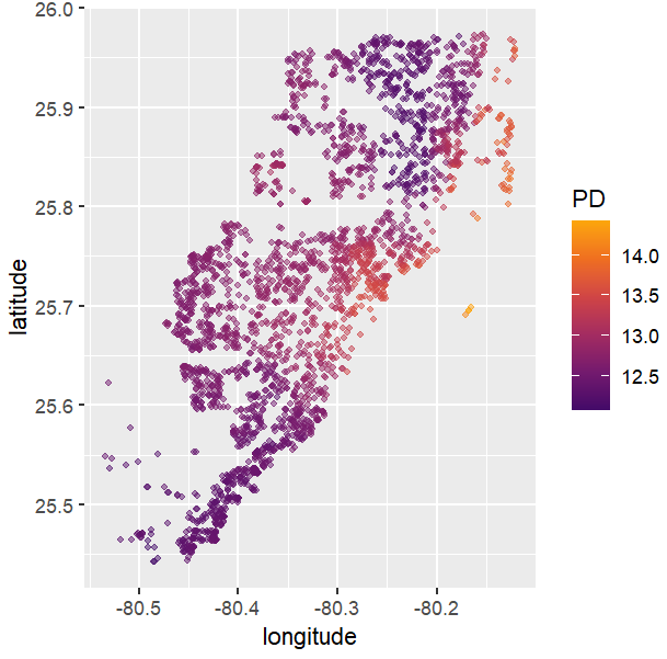
# Spatial plots
g <- unique(X_valid[, coord])
pp <- partial_dep(fit, v = coord, X = X_valid, grid = g)
plot(pp, d2_geom = "point", alpha = 0.5, size = 1) + 
  coord_equal()

# Takes some seconds because it generates the last plot per structure quality
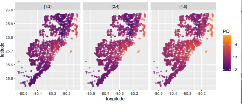
partial_dep(fit, v = coord, X = X_valid, grid = g, BY = "structure_quality") |>
  plot(pp, d2_geom = "point", alpha = 0.5) +
  coord_equal()
)

Results summarized by plots

Permutation importance

H-Statistics

Let’s now move on to interaction statistics.

Figure 4: Use “zero = FALSE” to drop variable (pairs) with value 0.

PDPs and ICEs

Figure 5: A partial dependence plot of living area.

Figure 6: Stratification shows indeed: no interactions between structure quality and living area.

Figure 7: ICE plots also show no interations with any other feature. The interaction constraints of XGBoost did a good job.

Figure 8: This two-dimensional PDP evaluated over all unique coordinates shows a realistic profile of house prices in Miami Dade County (mind the log scale).

Figure 8: Same, but grouped by structure quality (5 is best). Since there is no interaction between location and structure quality, the plots are just shifted versions of each other. (You can’t really see it on the plots.)

Naive Benchmark

All methods in {hstats} are optimized for speed. But how fast are they compared to other implementations? Note that: this is just a simple benchmark run on a Windows notebook with Intel i7-8650U CPU.

Note that {iml} offers a parallel backend, but we could not make it run with XGBoost and Windows. Let me know how fast it is using parallelism and Linux!

Setup + benchmark on permutation importance

Always using the full validation dataset and 10 repetitions.

library(iml)  # Might benefit of multiprocessing, but on Windows with XGB models, this is not easy
library(DALEX)
library(ingredients)
library(flashlight)
library(bench)

set.seed(1)

# iml
predf <- function(object, newdata) predict(object, data.matrix(newdata[x]))
mod <- Predictor$new(fit, data = as.data.frame(X_valid), y = y_valid, 
                     predict.function = predf)

# DALEX
ex <- DALEX::explain(fit, data = X_valid, y = y_valid)

# flashlight (my slightly old fashioned package)
fl <- flashlight(
  model = fit, data = valid, y = "log_price", predict_function = predf, label = "lm"
)
  
# Permutation importance: 10 repeats over full validation data (~2700 rows)
bench::mark(
  iml = FeatureImp$new(mod, n.repetitions = 10, loss = "mse", compare = "difference"),
  dalex = feature_importance(ex, B = 10, type = "difference", n_sample = Inf),
  flashlight = light_importance(fl, v = x, n_max = Inf, m_repetitions = 10),
  hstats = perm_importance(fit, X = X_valid, y = y_valid, m_rep = 10, verbose = FALSE),
  check = FALSE,
  min_iterations = 3
)

# expression      min   median `itr/sec` mem_alloc `gc/sec` n_itr  n_gc total_time
# iml           1.58s    1.58s     0.631   209.4MB    2.73      3    13      4.76s
# dalex      566.21ms 586.91ms     1.72     34.6MB    0.572     3     1      1.75s
# flashlight 587.03ms 613.15ms     1.63     27.1MB    1.63      3     3      1.84s
# hstats     353.78ms 360.57ms     2.79     27.2MB    0         3     0      1.08s

{hstats} is about 30% faster as the second, {DALEX}.

Partial dependence

Here, we study the time for crunching partial dependence of a continuous feature and a discrete feature.

# Partial dependence (cont)
v <- "tot_lvg_area"
bench::mark(
  iml = FeatureEffect$new(mod, feature = v, grid.size = 50, method = "pdp"),
  dalex = partial_dependence(ex, variables = v, N = Inf, grid_points = 50),
  flashlight = light_profile(fl, v = v, pd_n_max = Inf, n_bins = 50),
  hstats = partial_dep(fit, v = v, X = X_valid, grid_size = 50, n_max = Inf),
  check = FALSE,
  min_iterations = 3
)
# expression      min   median `itr/sec` mem_alloc `gc/sec` n_itr  n_gc total_time
# iml           1.11s    1.13s     0.887   376.3MB     3.84     3    13      3.38s
# dalex      782.13ms 783.08ms     1.24    192.8MB     2.90     3     7      2.41s
# flashlight 367.73ms  372.5ms     2.68     67.9MB     2.68     3     3      1.12s
# hstats     220.88ms  222.5ms     4.50     14.2MB     0        3     0   666.33ms
 
# Partial dependence (discrete)
v <- "structure_quality"
bench::mark(
  iml = FeatureEffect$new(mod, feature = v, method = "pdp", grid.points = 1:5),
  dalex = partial_dependence(ex, variables = v, N = Inf, variable_type = "categorical", grid_points = 5),
  flashlight = light_profile(fl, v = v, pd_n_max = Inf),
  hstats = partial_dep(fit, v = v, X = X_valid, n_max = Inf),
  check = FALSE,
  min_iterations = 3
)
# expression      min   median `itr/sec` mem_alloc `gc/sec` n_itr  n_gc total_time
# iml            90ms     96ms     10.6    13.29MB     7.06     3     2      283ms
# dalex       170.6ms  174.4ms      5.73   20.55MB     2.87     2     1      349ms
# flashlight   40.8ms   43.8ms     23.1     6.36MB     2.10    11     1      476ms
# hstats       23.5ms   24.4ms     40.6     1.53MB     2.14    19     1      468ms

{hstats} is 1.5 to 2 times faster than {flashlight}, and about four times as fast as the other packages. It’s memory foodprint is much lower.

H-statistics

How fast can overall H-statistics be computed? How fast can it do pairwise calculations?

{DALEX} does not offer these statistics yet. {iml} was the first model-agnostic implementation of H-statistics I am aware of. It uses quantile approximation by default, but we purposely force it to calculate exact, in order to compare the numbers. Thus, we made it slower than it actually is.

# H-Stats -> we use a subset of 500 rows
X_v500 <- X_valid[1:500, ]
mod500 <- Predictor$new(fit, data = as.data.frame(X_v500), predict.function = predf)
fl500 <- flashlight(fl, data = as.data.frame(valid[1:500, ]))

# iml  # 225s total, using slow exact calculations
system.time(  # 90s
  iml_overall <- Interaction$new(mod500, grid.size = 500)
)
system.time(  # 135s for all combinations of latitude
  iml_pairwise <- Interaction$new(mod500, grid.size = 500, feature = "latitude")
)

# flashlight: 14s total, doing only one pairwise calculation, otherwise would take 63s
system.time(  # 12s
  fl_overall <- light_interaction(fl500, v = x, grid_size = Inf, n_max = Inf)
)
system.time(  # 2s
  fl_pairwise <- light_interaction(
    fl500, v = coord, grid_size = Inf, n_max = Inf, pairwise = TRUE
  )
)

# hstats: 3s total
system.time({
  H <- hstats(fit, v = x, X = X_v500, n_max = Inf)
  hstats_overall <- h2_overall(H, squared = FALSE, zero = FALSE)
  hstats_pairwise <- h2_pairwise(H, squared = FALSE, zero = FALSE)
}
)

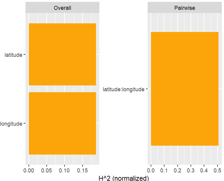
# Overall statistics correspond exactly
iml_overall$results |> filter(.interaction > 1e-6)
#     .feature .interaction
# 1:  latitude    0.2458269
# 2: longitude    0.2458269

fl_overall$data |> subset(value > 0, select = c(variable, value))
#   variable  value
# 1 latitude  0.246
# 2 longitude 0.246

hstats_overall
# longitude  latitude 
# 0.2458269 0.2458269 

# Pairwise results match as well
iml_pairwise$results |> filter(.interaction > 1e-6)
#              .feature .interaction
# 1: longitude:latitude    0.3942526

fl_pairwise$data |> subset(value > 0, select = c(variable, value))
# latitude:longitude 0.394

hstats_pairwise
# latitude:longitude 
# 0.3942526

{hstats} is about four times as fast as {flashlight}.
Since one often want to study relative and absolute H-statistics, in practice, the speed-up would be about a factor of eight.
In multi-classification/multi-output settings with m categories, the speed-up would be even m times larger.
The fast approximation via quantile binning is again a factor of four faster. The difference would diminish if we would calculate many pairwise or three-way H-statistics.
Forcing all three packages to calculate exact statistics, all results match.

Wrap-Up

{hstats} is much faster than other XAI packages, at least in our use-case. This includes H-statistics, permutation importance, and partial dependence. Note that making good benchmarks is not my strength, so forgive any bias in the results.
The memory foodprint is lower as well.
With multivariate output, the potential is even larger.
H-Statistics match other implementations.

Try it out!

The full R code in one piece is here.

Comments

3 responses to “Interactions – where are you?”

2023-11-01

Wolf

Nice! Looks very interesting.
Concerning benchmarks: I’d use bench::mark() now. It is more explicit about gc (garbage collection), which can influence measurements considerably.

1. 2023-11-12
  
  Michael Mayer
  
  Thanks a lot for the hint. I have now changed the post to use {bench}. Memory foodprints are very useful!
  
2023-11-11

Michael Mayer

Fair point, thanks. I will try to switch to {bench} for my next benchmark!

Interactions – where are you?

1. Example

Results summarized by plots

Permutation importance

H-Statistics

PDPs and ICEs

Naive Benchmark

Setup + benchmark on permutation importance

Partial dependence

H-statistics

Wrap-Up

Comments

3 responses to “Interactions – where are you?”

Leave a Reply Cancel reply

More posts

Introducing LightSHAP

Key improvements in shapviz and kernelshap

Update of Swiss Mortality

Model Diagnostics: Statistics vs Machine Learning