TLDR: The scipy 1.7.0 release introduced Wright’s generalized Bessel function in the Python ecosystem. It is an important ingredient for the density and log-likelihood of Tweedie probabilty distributions. In this last part of the trilogy I’d like to point out why it was important to have this function and share the endeavor of implementing this inconspicuous but highly intractable special function. The fun part is exploiting a free parameter in an integral representation, which can be optimized by curve fitting to the minimal arc length.
This trilogy celebrates the 40th birthday of Tweedie distributions in 2024 and highlights some of their very special properties.
Tweedie Distributions
As pointed out in part I and part II, the family of Tweedie distributions is a very special one with outstanding properties. They are central for estimating expectations with GLMs. The probability distributions have mainly positive (non-negative) support and are skewed, e.g. Poisson, Gamma, Inverse Gaussian and compound Poisson-Gamma.
As members of the exponential dispersion family, a slight extension of the exponential family, the probability density can be written as
\begin{align*}
f(y; \theta, \phi) &= c(y, \phi) \exp\left(\frac{y\theta - \kappa(\theta)}{\phi}\right)
\\
\kappa(\theta) &= \kappa_p(\theta) = \frac{1}{2-p}((1-p)\theta)^{\frac{2-p}{1-p}}
\end{align*}
It is often more instructive to parametrise the distribution with p, \mu and \phi
\begin{align*}
\theta &= \begin{cases}
\frac{\mu^{1-p}}{1-p}\,,\quad p\neq 1\\
\log(\mu)\,,\quad p=1
\end{cases}
\\
\kappa(\theta) &= \begin{cases}
\frac{\mu^{2-p}}{2-p}\,,\quad p\neq 2\\
\log(\mu)\,,\quad p=2
\end{cases}
\end{align*}
and write
\begin{align*}
Y &\sim \mathrm{Tw}_p(\mu, \phi)
\end{align*}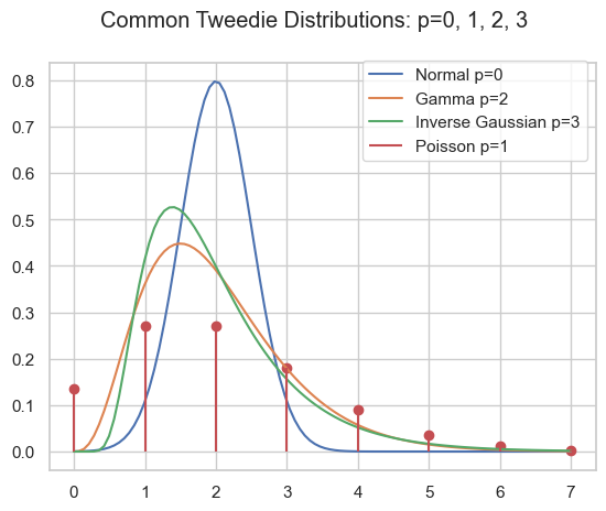
Compound Poisson Gamma
A very special domain for the power parameter is between Poisson and Gamma: 1<p<2. This range results in the Compound Poisson distribution which is suitable if you have a random count process and if each count itself has a random amount. A well know example is insurance claims. Typically, there is a random number of insurance claims, and each and every claim has a random amount of claim costs.
\begin{align*}
N &\sim \mathrm{Poisson}(\lambda)\\
X_i &\sim \mathrm{Gamma}(a, b)\\
Y &= \sum_{i=0}^N X_i \sim \mathrm{CompPois}(\lambda, a, b)
\end{align*}
For Poisson count we have \operatorname{E}[N]=\lambda and \operatorname{Var}[N]=\lambda=\operatorname{E}[N], for the Gamma amount \operatorname{E}[X]=\frac{a}{b}\operatorname{Var}[X]=\frac{a}{b^2}=\frac{1}{a}\operatorname{E}[X]^2. For the compound Poisson-Gamma variable, we obtain
\begin{align*}
\operatorname{E}[Y] &= \operatorname{E}[N] \operatorname{E}[X] = \lambda\frac{a}{b}=\mu\\
\operatorname{Var}[Y] &=  \operatorname{Var}[N] \operatorname{E}[X]^2 +  \operatorname{E}[N] \operatorname{Var}[X] =  \phi \mu^p\\
p &= \frac{a + 2}{a+1} \in (1, 2)\\
\phi &= \frac{(\lambda a)^{1-p}}{(p-1)b^{2-p}}
\end{align*}
What’s so special here is that there is a point mass at zero, i.e., P(Y=0)=\exp(-\frac{\mu^{2-p}}{\phi(2-p)}) > 0. Hence, it is a suitable distribution for non-negative quantities with some exact zeros.
Code
import matplotlib.pyplot as plt
import numpy as np
from scipy.special import wright_bessel
def cpg_pmf(mu, phi, p):
"""Compound Poisson Gamma point mass at zero."""
return np.exp(-np.power(mu, 2 - p) / (phi * (2 - p)))
def cpg_pdf(x, mu, phi, p):
"""Compound Poisson Gamma pdf."""
if not (1 < p < 2):
raise ValueError("1 < p < 2 required")
theta = np.power(mu, 1 - p) / (1 - p)
kappa = np.power(mu, 2 - p) / (2 - p)
alpha = (2 - p) / (1 - p)
t = ((p - 1) * phi / x)**alpha
t /= (2 - p) * phi
a = 1 / x * wright_bessel(-alpha, 0, t)
return a * np.exp((x * theta - kappa) / phi)
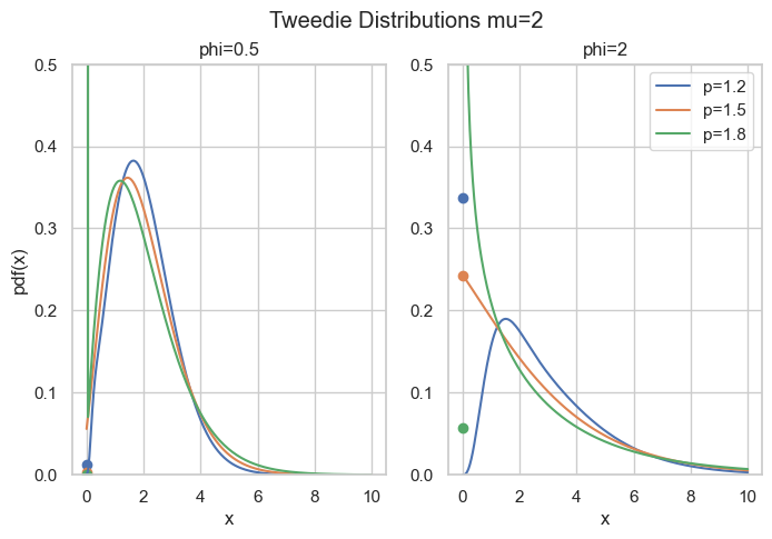
fig, axes = plt.subplots(ncols=2, figsize=[6.4 * 1.25, 4.8])
x = np.linspace(1e-9, 10, 200)
mu = 2
for p in [1.2, 1.5, 1.8]:
for i, phi in enumerate([0.5, 2]):
axes[i].plot(x, cpg_pdf(x=x, mu=mu, phi=phi, p=p), label=f"{p=}")
axes[i].scatter(0, cpg_pmf(mu=mu, phi=phi, p=p))
axes[i].set_ylim(0, 0.5)
axes[i].set_title(f"{phi=}")
if i > 0:
axes[i].legend()
else:
axes[i].set_ylabel("pdf(x)")
axes[i].set_xlabel("x")
fig.suptitle("Tweedie Distributions mu=2")The rest of this post is about how to compute the density for this parameter range. The easy part is \exp\left(\frac{y\theta - \kappa(\theta)}{\phi}\right) which can be directly implemented. The real obstacle is the term c(y, \phi) which is given by
\begin{align*}
c(y, \phi) &= \frac{\Phi(-\alpha, 0, t)}{y}
\\
\alpha &= \frac{2 - p}{1 - p}
\\
t &= \frac{\left(\frac{(p - 1)\phi}{y}\right)^{\alpha}}{(2-p)\phi}
\end{align*}
This depends on Wright’s (generalized Bessel) function \Phi(a, b, z) as introduced in a 1933 paper by E. Wright.
Wright’s Generalized Bessel Function
According to DLMF 10.46, the function is defined as
\begin{equation*}
\Phi(a, b, z) = \sum_{k=0}^{\infty} \frac{z^k}{k!\Gamma(ak+b)}, \quad a > -1, b \in R, z \in C
\end{equation*}
which converges everywhere because it is an entire function. We will focus on the positive real axis z=x\geq 0 and the range a\geq 0, b\geq 0 (note that a=-\alpha \in (0,\infty) for 1<p<2). For the compound Poisson-Gamma, we even have b=0.
Implementation of such a function as done in scipy.stats.wright_bessel, even for the restricted parameter range, poses tremendous challenges. The first one is that it has three parameters which is quite a lot. Then the series representation above, for instance, can always be used, but depending on the parameters, it will require a huge amount of terms, particularly for large x. As each term involves the Gamma function, this becomes expensive very fast. One ends up using different representations and strategies for different parameter regions:
- Small
x: Taylor series according to definition - Small
a: Taylor series ina=0 - Large
x: Asymptotic series due to Wright (1935) - Large
a: Taylor series according to definition for a few terms around the approximate maximum termk_{max}due to Dunn & Smyth (2005) - General: Integral represantation due to Luchko (2008)
Dunn & Smyth investigated several evaluation strategies for the simpler Tweedie density which amounts to Wright’s functions with b=0, see Dunn & Smyth (2005). Luchko (2008) lists most of the above strategies for the full Wright’s function.
Note that Dunn & Smyth (2008) provide another strategy to evaluate the Tweedie distribution function by means of the inverse Fourier transform. This does not involve Wright’s function, but also encounters complicated numerical integration of oscillatory functions.
The Integral Representation
This brings us deep into complex analysis: We start with Hankel’s contour integral representation of the reciprocal Gamma function.
\begin{equation*}
\frac{1}{\Gamma(z)} = \frac{1}{2\pi i} \int_{Ha^-} \zeta^{-z} e^\zeta \; d\zeta
\end{equation*}
with the Hankel path Ha^- from negative infinity (A) just below the real axis, counter-clockwise with radius \epsilon>0 around the origin and just above the real axis back to minus infinity (D).

In principle, one is free to choose any such path with the same start (A) and end point (D) as long as one does not cross the negative real axis. One usually lets the AB and CD be infinitesimal close to the negative real line. Very importantly, the radius \epsilon>0 is a free parameter! That is real magic🪄
By interchanging sum and integral and using the series of the exponential, Wright’s function becomes
\begin{align*}
\Phi(a, b, z) &= \sum_{k=0}^{\infty} \frac{z^k}{k!} \frac{1}{2\pi i} \int_{Ha^-} \zeta^{-(ak+b)} e^\zeta \; d\zeta
\\
&= \frac{1}{2\pi i} \int_{Ha^-} \zeta^{-b} e^{\zeta + z\zeta^{-a}} \; d\zeta
\end{align*}
Now, one needs to do the tedious work and split the integral into the 3 path sections AB, BC, CD. Putting AB and CD together gives an integral over K, the circle BC gives an integral over P:
\begin{align*}
\Phi(a, b, x) &= \frac{1}{\pi} \int_{\epsilon}^\infty K(a, b, x, r) \; dr
\\
 &+ \frac{\epsilon^{1-b}}{\pi} \int_0^\pi P(\epsilon, a, b, x, \varphi) \; d\varphi
\\
K(a, b, x, r) &= r^{-b}\exp(-r + x  r^{-a} \cos(\pi a))
\\
&\quad \sin(x \cdot r^{-a} \sin(\pi a) + \pi b)
\\
P(\epsilon, a, b, x, \varphi) &= \exp(\epsilon \cos(\varphi) + x  \epsilon^{-a}\cos(a \varphi))
\\
&\quad \cos(\epsilon \sin(\varphi) - x \cdot \epsilon^{-a} \sin(a \varphi) + (1-b) \varphi)
\end{align*}
What remains is to carry out the numerical integration, also known as quadrature. While this is an interesting topic in its own, let’s move to the magic part.
Arc Length Minimization
If you have come so far and say, wow, puh, uff, crazy, 🤯😱 Just keep on a little bit because here comes the real fun part🤞
It turns out that most of the time, the integral over P is the most difficult. The worst behaviour an integrand can have is widely oscillatory. Here is one of my favorite examples:
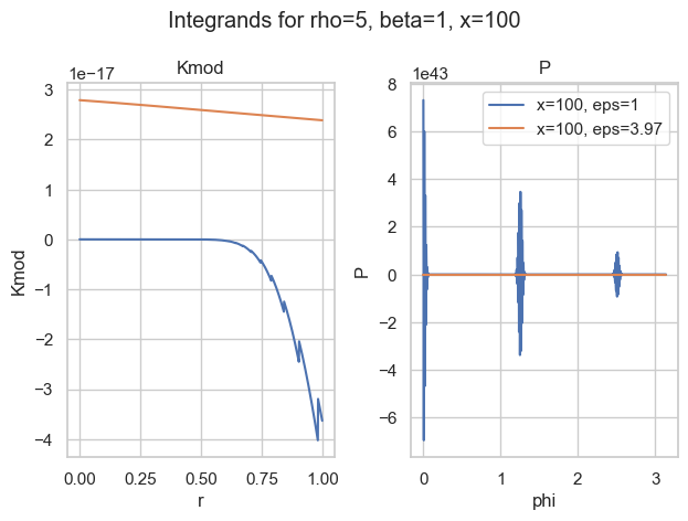
With the naive choice of \epsilon=1, both integrands (blue) are—well—crazy. There is basically no chance the most sophisticated quadrature rule will work. And then look at the other choice of \epsilon\approx 4. Both curves seem well behaved (for P, we would need a closer look).
So the idea is to find a good choice of \epsilon to make P well behaved. Well behaved here means most boring, if possible a straight line. What makes a straight line unique? In flat space, it is the shortest path between two points. Therefore, well behaved integrands have minimal arc length. That is what we want to minimize.
The arc length S from x=a to x=b of a 1-dimensional function f is given by
\begin{equation*}
S = \int_a^b \sqrt{1 + f^\prime(x)^2} \; dx
\end{equation*}
Instead of f=P, we only take the oscillatory part of P and approximate the arc length as f(\varphi)=f(\varphi) = \epsilon \sin(\varphi) - x \epsilon^{-\rho} \sin(\rho \varphi) + (1-\beta) \varphi. For a single parameter point a, b, z this looks like
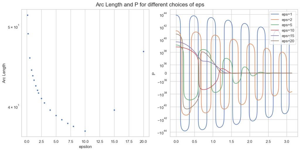
Note the logarithmic y-scale for the right plot of P. The optimal \epsilon=10 is plotted in red and behaves clearly better than smaller values of \epsilon.
What remains to be done for an actual implementation is
- Calculate minimal
\epsilonfor a large grid of valuesa, b, x. - Choose a function with some parameters.
- Curve fitting (so again optimisation): Fit this function to the minimal
\epsilonof the grid via minimising least squares. - Implement some quadrature rules and use this choice of
\epsilonin the hope that it intra- and extrapolates well.
This strategy turns out to work well in practice and is implemented in scipy. As the parameter space of 3 variables is huge, the integral representation breaks down in certain areas, e.g. huge values of \epsilon where the integrands just overflow numerically (in 64-bit floating point precision). But we have our other evaluation strategies for that.
Conclusion
An extensive notebook for Wright’s function, with all implementation strategies can be found here.
After an adventurous journey, we arrived at one implementation strategy of Wright’s generalised Bessel function, namely the integral representation. The path went deep into complex analysis and contour integration, then further to the arc length of a function and finally curve fitting via optimisation. I am really astonished how connected all those different areas of mathematics can be.
Wright’s function is the missing piece to compute full likelihoods and probability functions of the Tweedie distribution family and is now available in the Python ecosystem via scipy.
We are at the very end of this Tweedie trilogy. I hope it has been entertaining and it has become clear why Tweedie deserves to be celebrated.
Further references:
- Delong, Ł., Lindholm, M. & Wüthrich, M.V. “Making Tweedie’s compound Poisson model more accessible”. Eur. Actuar. J. 11, 185–226 (2021). https://doi.org/10.1007/s13385-021-00264-3
- Wright E.M. 1933. “On the coefficients of power series having essential singularities”. J. London Math. Soc. 8: 71–79. https://doi.org/10.1112/jlms/s1-8.1.71
- Wright, E. M. 1935, “The asymptotic expansion of the generalized Bessel”, function. Proc. London Math. Soc. (2) 38, pp. 257–270. https://doi.org/10.1112/plms/s2-38.1.257
- Dunn, P.K., Smyth, G.K. “Series evaluation of Tweedie exponential dispersion model densities”. Stat Comput 15, 267–280 (2005). https://doi.org/10.1007/s11222-005-4070-y
- Dunn, P.K., Smyth, G.K. “Evaluation of Tweedie exponential dispersion model densities by Fourier inversion”. Stat Comput 18, 73–86 (2008). https://doi.org/10.1007/s11222-007-9039-6
- Luchko, Y. F. (2008), “Algorithms for Evaluation of the Wright Function for the Real Arguments’ Values”, Fractional Calculus and Applied Analysis 11(1). https://eudml.org/doc/11309
Note a slight misprint in the integrand P.