Tag: data science

In this post, we explore the topic of gap safe screening rules from convex optimisation and their impact on Lasso and ElasticNet in scikit-learn.

The Lasso in convex optimisation

As ordinary least squares the Lasso model consists of predictions X\cdot\beta with feature matrix X \in \mathbb{R}^{n, p} and fitted coefficients \beta. Given observations y, the coefficients are estimated by solving the convex optimisation problem

\beta^\star = \argmin_\beta \left( P(\beta)=\frac{1}{2n} \lVert y-X\beta\rVert_2^2 + \alpha \lVert\beta\rVert_1 \right)

This is called the primal formulation of the Lasso. For simplicity, we ignore an intercept (bias) term and assume that X and y are mean centered.

The major tool we need in this post is the dual formulation:

\nu^\star = \argmax_{\{\nu: \lVert X'\nu\rVert_\infty \leq n\alpha\} } \left( D(\nu)=-\frac{1}{2n} \lVert \nu\rVert_2^2 + \frac{1}{n} y\cdot \nu \right)

This is an optimisation problem in terms of the dual variable \nu which has to be in the dual feasible set \{\nu: \lVert X'\nu\rVert_\infty \leq n\alpha\}.

Now the wonderful theory of convex optimisation states:

D(\nu) \leq P(\beta^\star)

G(\beta, \nu) =P(\beta) - D(\nu) \geq P(\beta) - P(\beta^\star)\geq 0

D(\nu^\star) = P(\beta^\star)

y - X\beta^\star = \nu^\star

Both weak and strong duality hold for the Lasso. Weak duality acts as a lower bound for the optimal primal value. The duality gap is therefore a conservative proxy for how close a current iteration is from the optimum. It is a very good stopping criterion for algorithms. Other optimisation problems would wish to have such a good guarantee when to stop iterating.

Screening rules in coordinate descent

The main algorithm to solver the Lasso is coordinate descent as implemented in many packages:

• R: glmnet
• Python: scikit-learn, Celer, skglm

The core idea of coordinate descent is very simple:

1. Choose a coordinate j (a.k. feature or column) of X.
2. Minimize P w.r.t. \beta_j while keeping all the other coefficients constant.
3. Repeat steps 1 and 2 until convergence (e.g. the dual gap is smaller than a user given tolerance).

The second step even has a short closed form solution, called soft-thresholding, for the Lasso which makes it ideal for implementations.

Whenever you have an iterate \beta, you can calculate a feasible dual point \nu as follows:

1. Set \nu = y - X\beta.
2. If \nu is not feasible, rescale it by its dual norm: \nu \rightarrow \nu \frac{n\alpha}{\lVert X'\nu\rVert_\infty}.

The last ingredient are screening rules. The basic idea is the following: One important property of the Lasso is that it is able to set coefficients exactly to zero. The stronger the penalty \alpha the more likely that some coefficients vanish. While cycling through the coordinates, safe screening rules allow to identify whether a coordinate can be set to zero. There are also non-safe screening rules which rely on heuristics. They later must check again.

The practical most relevant gap safe screening rule is the one based on a sphere test:

\frac{n\alpha-\lvert x_j\cdot \nu \rvert}{\rVert x_j\rVert_2}>\sqrt{2nG(\beta,\nu)} \Rightarrow \beta_j=0

I implemented these gap safe screening rules for the scikit-learn estimators in pull requests #31882, #31986, #31987 and #32014. Together with some further nice improvements they became available with scikit-learn version 1.8, see the release highlights.

Benchmark

Enough theory, time for some coding and benchmarks. Was is worth the implementation? In the following mini-benchmark, I intentionally called the estimators as a user would do. I could have just called the underlying algorithms to avoid input validation and transformation, I could have set fit_intercept=False. The improvements therefore show what a user could expect.

The first benchmark is on the Leukemia dataset with only 72 observations but 7,129 features. Here, a whole path of alpha values is computed for three different values of the stopping tolerance.

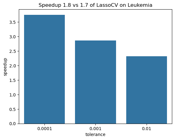
This shows a nice speedup of 2-4 times!

The second small benchmark is with the finance dataset, a.k.a. E2006-log1p with 16,087 observations and 4,272,227 features; this is quite large. The data is given as sparse matrix with a density of 0.14% (0.14% of entries have a value, the other entries are implicitly considered zero) which runs a different code path but with the same coordinate descent algorithm. This time, Celer and skglm are also compared.

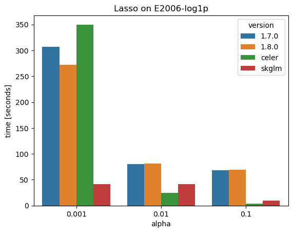
Two points seem worth noticing:

• The gap safe screening rules of scikit-learn 1.8 show little to no improvement over version 1.7 without screening rules.
• Celer and skglm are significantly faster for larger penalties, skglm is always faster.

Note that Celer and skglm use different refinements of the underlying coordinate descent algorithms.

The full code is available as jupyter notebook.

Conclusion

I would like to close this post with a few remarks:

• Results from theory like the gap safe screening rule can have a huge impact on algorithms.
• From the publication of “Mind the duality gap” until their release in scikit-learn was a gap of 10 years.
• Alexandre Gramfort is one of the very few people (to my knowledge the only one) who has contributed code to scikit-learn (he is a core contributor since the beginnings) and who published a paper that was implemented.
• There is ongoing work to bring these improvements of L1-solvers to logistic regression and other GLMs. Give your 👍 to pull request #33160.

Further references:

• Kim, S.-J., Koh, K., Lustig, M., Boyd, S., and Gorinevsky,D. “An Interior-Point Method for Large-Scale ℓ1-Regularized Least Squares”. IEEE J. Sel. Topics Signal Process., 1(4):606–617, 2007. https://doi.org/10.1109/JSTSP.2007.910971
• Friedman, J., Hastie, T. J., Höfling, H., and Tibshirani, R. “Pathwise coordinate optimization”. Ann. Appl. Stat., 1(2):302–332, 2007. https://doi.org/10.1214/07-AOAS131
• Fercoq, O., Gramfort, A., and Salmon, J. “Mind the duality gap: safer rules for the lasso”. In ICML, pp. 333–342, 2015. https://doi.org/10.48550/arXiv.1505.03410
• Zou, H. and Hastie, T. “Regularization and variable selection via the elastic net”. J. Roy. Statist. Soc. Ser. B, 67(2): 301–320, 2005. https://doi.org/10.1111/j.1467-9868.2005.00527.x
• Dünner, C., Forte, S., Takác, M. and Jaggi, M. “Primal-Dual Rates and Certificates”. In ICML 2016 – Proceedings of the 33th International Conference on Machine Learning, pages 783–792, 2016. https://doi.org/10.48550/arXiv.1602.05205

Appendix: Elastic Net

The Elastic Net is an extension of the Lasso that adds an L2-penalty:

P(\beta)=\frac{1}{2n} \lVert y-X\beta\rVert_2^2 + \alpha_1 \lVert\beta\rVert_1 + \frac{\alpha_2}{2} \lVert\beta\rVert_2^2

Very interestingly, there are two different dual formulations for it. There is the one that can be derived by extending p artificial observations to X and y, see Zou & Hastie 2005:

\begin{align*}
X \rightarrow \tilde{X}&=\begin{pmatrix}X\\ \sqrt{n\alpha_2}\,\mathbb{1}_p\end{pmatrix}\,,\quad
y \rightarrow \tilde{y}= \begin{pmatrix}y\\ \mathbb{0}_p\end{pmatrix}
\\
P(\beta)&=-\frac{1}{2n} \lVert \tilde{y}-\tilde{X}\beta\rVert_2^2 + \alpha_1\lVert \beta\rVert_1
\\
\nu \rightarrow\tilde{\nu} &= \begin{pmatrix}\nu\\ \sqrt{n\alpha_2}\beta\end{pmatrix}\
\\
D(\nu)&=-\frac{1}{2n} \lVert \nu\rVert_2^2 + \frac{1}{n} y\cdot \nu - \frac{\alpha_2}{2}\lVert \nu\rVert_2^2
\\
\mathrm{feasible\, set}&=\{\nu: \lVert X'\nu - n\alpha_2\beta\rVert_\infty \leq n\alpha_1\}
\end{align*}

And dual can be derived by direct computation starting with the primal, see also Dünner et al 2016:

\begin{align*}
D(\nu) =& -\frac{1}{2n} \lVert \nu\rVert_2^2 + \frac{1}{n} y\cdot \nu
\\
&- \frac{1}{2n^2\alpha_2}
-\sum_j \left( \lvert x_j\cdot\nu\rvert_2 - n\alpha_1\right)_+^2 \,,\quad \alpha_2>0
\\
&\mathrm{feasible\, set}=\mathbb{R}\end{align*}

Here, (x)_+=\max(x,0) denotes the positive part. Very surprisingly, the dual feasible set equals the real numbers, no restrictions! The disadvantage is that this formulation only holds for \alpha_2>0.

The two different duals result in two different dual gaps for the Elastic Net. It actually makes quite a difference as investigated in scikit-learn issue #22836.