Category: Data

  • Key improvements in shapviz and kernelshap

    SHAP interaction strength for the XGBoost model (single variables reflect SHAP main effect strength).

    Our two sister packages are continuously being improved. A brief summary of the latest changes:

    shapviz (v0.10.2)

    1. Identical axes, axis titles and color bars are now collected across dependence plots.
    2. Dependence plots have received arguments share_y=FALSE and ylim=NULL for better comparability across subplots.
    3. New visualization for SHAP interaction strenght via sv_interaction(kind="bar"). It shows mean absolute SHAP interaction/main effects, where the interaction values are multiplied by two for symmetry.

    kernelshap (v0.9.1)

    1. permshap() now offers a balanced sampling version which iterates until convergence and returns standard errors. It is used by default when the model has more than eight features, or by setting exact=FALSE.
    2. Fixed an error in kernelshap() which made the resulting values slightly off for models with interactions of order three or higher. Now, the exact version returns the same values as exact permutation SHAP and agrees with the exact explainer in Python’s shap package.

    Illustrating sampling permutation SHAP

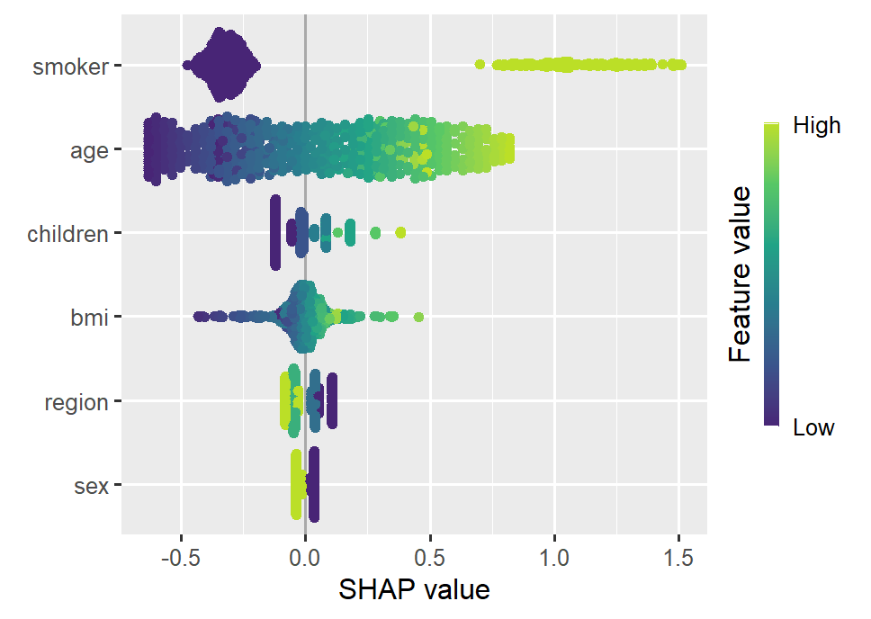
    Let’s use a beautiful dataset on medical costs to fit a log-linear Gamma GLM with interactions between all features and smoking, and explain it by SHAP on log prediction (= linear) scale.

    Since the model does not contain interactions of order above 2, the SHAP values perfectly reconstruct the estimated model coefficients, see our recent paper on https://arxiv.org/abs/2508.12947 for a proof.

    Smoking and age are the most important features. Some strong interactions with smoking are visible.

    library(xgboost)
    library(ggplot2)
    library(patchwork)
    library(shapviz)
    library(kernelshap)
    
    options(shapviz.viridis_args = list(option = "D", begin = 0.1, end = 0.9))
    
    set.seed(1)
    
    # https://github.com/stedy/Machine-Learning-with-R-datasets
    df <- read.csv("https://raw.githubusercontent.com/stedy/Machine-Learning-with-R-datasets/refs/heads/master/insurance.csv")
    
    # Gamma GLM with interactions
    fit_glm <- glm(charges ~ . * smoker, data = df, family = Gamma(link = "log"))
    
    # Use SHAP to explain
    xvars <- c("age", "sex", "bmi", "children", "smoker", "region")
    X_explain <- head(df[xvars], 500)
    
    # The new sampling permutation algo (forced with exact = FALSE)
    shap_glm <- permshap(fit_glm, X_explain, exact = FALSE, seed = 1) |>
      shapviz()
    
    sv_importance(shap_glm, kind = "bee")
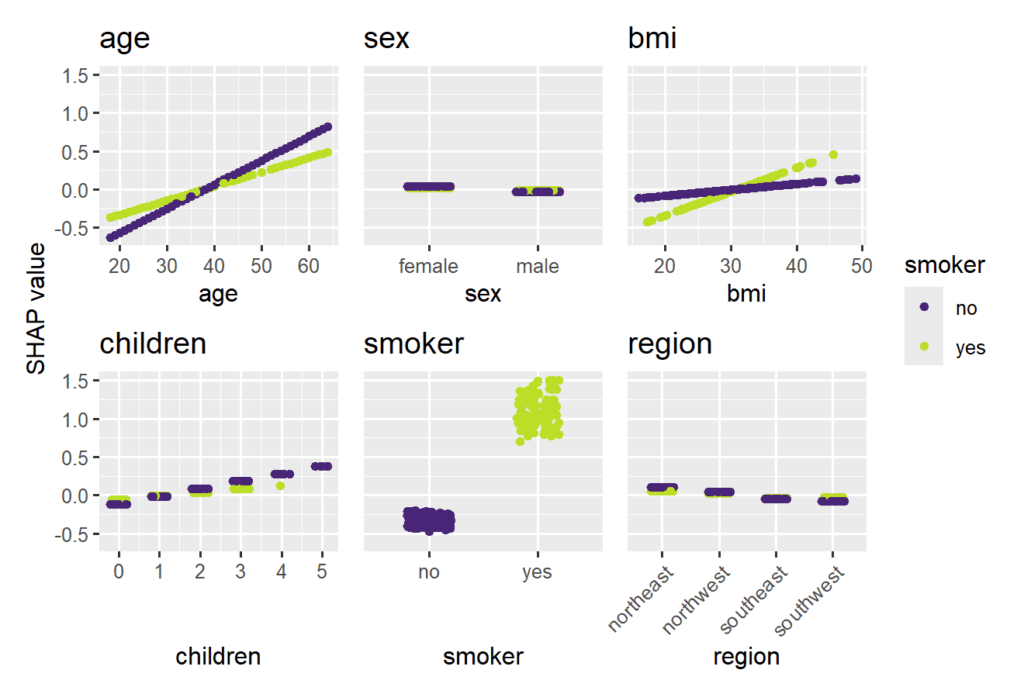
    
    sv_dependence(
      shap_glm,
      v = xvars,
      share_y = TRUE,
      color_var = "smoker"
    )
    
    SHAP beeswarm plot of the Gamma GLM
    SHAP dependence plots of the Gamma GLM, using “smoking” on the color scale

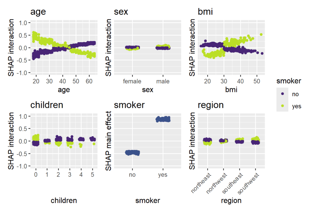
    Illustrating SHAP interaction strength

    As a second example, we sloppily fit an XGBoost model with Gamma deviance loss to illustrate some of the SHAP interaction functionality of {shapviz}. As with the GLM, the SHAP values are being calculated on log scale.

    For the sake of brevity, we focus on plots visualizing SHAP interactions. In practice, make sure to use a clean train/test/(x-)validation and tuning approach.

    The strongest interaction effects (smoker * age, smoker * bmi) are stronger than most main effects. Not all interactions seem natural.

    # XGBoost model (sloppily without tuning)
    X_num <- data.matrix(df[xvars])
    fit_xgb <- xgb.train(
      params = list(objective = "reg:gamma", learning_rate = 0.2),
      data = xgb.DMatrix(X_num, label = df$charges),
      nrounds = 100
    )
    
    shap_xgb <- shapviz(fit_xgb, X_pred = X_num, X = df, interactions = TRUE)
    
    # SHAP interaction/main-effect strength
    sv_interaction(shap_xgb, kind = "bar", fill = "darkred")
    
    # Study interaction/main-effects of "smoking"
    sv_dependence(
      shap_xgb,
      v = xvars,
      color_var = "smoker",
      ylim = c(-1, 1),
      interactions = TRUE
    ) + # we rotate axis labels of *last* plot, otherwise use &
      guides(x = guide_axis(angle = 45))
    
    SHAP interaction strength for the XGBoost model (single variables reflect SHAP main effect strength).
    SHAP interaction effects with smoking for the XGBoost model, including the main effect of smoking

    Keep an eye on these two packages for further improvements… 🙂

    R script

  • Fast Grouped Counts and Means in R

    Edited on 2025-05-01: Multiple improvements by Christian, especially on making Polars neater, DuckDB faster, and the plot easier to read.

    From time to time, the following questions pop up:

    1. How to calculate grouped counts and (weighted) means?
    2. What are fast ways to do it in R?

    This blog post presents a couple of approaches and then compares their speed with a naive (non-scientific!) benchmark.

    Base R

    There are many ways to calculate grouped counts and means in base R, e.g., aggregate(), tapply(), by(), split() + lapply(). In my experience, the fastest way is a combination of tabulate() and rowsum().

    # Make data
    set.seed(1)
    
    n <- 1e6
    
    y <- rexp(n)
    w <- runif(n)
    g <- factor(sample(LETTERS[1:3], n, TRUE))
    df <- data.frame(y = y, g = g, w = w)
    
    # Grouped counts
    tabulate(g)
    # 333469 333569 332962
    
    # Grouped means
    rowsum(y, g) / tabulate(g)
          [,1]
    # A 1.000869
    # B 1.001043
    # C 1.000445
    
    # Grouped weighted mean
    ws <- rowsum(data.frame(y = y * w, w), g)
    ws[, 1L] / ws[, 2L]
    # 1.0022749 1.0017816 0.9997058

    But: tabulate() ignores missing values. To avoid problems, create an explicit missing level via factor(x, exclude = NULL).

    Let’s turn to some other approaches.

    dplyr

    Not optimized for speed or memory, but the de-facto standard in data processing with R. I love its syntax.

    library(tidyverse)
    
    df <- tibble(df)
    
    # Grouped counts
    dplyr::count(df, g)
    
    # Grouped means
    df |>
      group_by(g) |>
      summarize(mean(y))
    
    # Grouped weighted means
    df |>
      group_by(g) |>
      summarize(sum(w * y) / sum(w))

    data.table

    Does not need an introduction. Since 2006 the package for fast data manipulation written in C.

    library(data.table)
    
    dt <- data.table(df)
    
    # Grouped counts (use keyby for sorted output)
    dt[, .N, by = g]
    #         g      N
    #    <fctr>  <int>
    # 1:      C 332962
    # 2:      B 333569
    # 3:      A 333469
    
    # Grouped means
    dt[, mean(y), by = g]
    
    # Grouped weighted means
    dt[, sum(w * y) / sum(w), by = g]
    dt[, weighted.mean(y, w), by = g]

    DuckDB

    Extremely powerful query engine / database system written in C++, with initial release in 2019, and R bindings since 2020. Allows larger-than-RAM calculations.

    library(duckdb)
    
    con <- dbConnect(duckdb())
    
    # only registers: duckdb_register(con, name = "df", df = df)
    dbWriteTable(con, name = "df", value = df)
    
    dbGetQuery(con, "SELECT g, COUNT(*) N FROM df GROUP BY g")
    dbGetQuery(con, "SELECT g, AVG(y) AS mean FROM df GROUP BY g")
    con |> 
      dbGetQuery(
      "
      SELECT g, SUM(y * w) / sum(w) as wmean
      FROM df
      GROUP BY g
      "
      )
    #   g     wmean
    # 1 A 1.0022749
    # 2 B 1.0017816
    # 3 C 0.9997058

    collapse

    C/C++-based package for data transformation and statistical computing. {collapse} was initially released on CRAN in 2020. It can do much more than grouped calculations, check it out!

    library(collapse)
    
    fcount(g)
    fnobs(g, g) # Faster and does not need memory, but ignores missing values
    fmean(y, g = g)
    fmean(y, g = g, w = w)
    #         A         B         C
    # 1.0022749 1.0017816 0.9997058

    Polars

    R bindings of the fantastic Polars project that started in 2020. First R release in 2022. Currently under heavy revision.

    The current package is not up-to-date with the main project, thus we expect the revised version (available in this branch) to be faster.

    # Sys.setenv(NOT_CRAN = "true")
    # install.packages("polars", repos = "https://community.r-multiverse.org")
    library(polars)
    
    dfp <- as_polars_df(df)
    
    # Grouped counts
    dfp$get_column("g")$value_counts()
    # Faster, but eats more memory
    dfp$select("g")$with_columns(pl$lit(1L))$group_by("g")$sum()
    
    # Grouped means
    (
      dfp
      $group_by("g")
      $agg(pl$col("y")$mean())
    )
    
    # Grouped weighted means
    (
      dfp
      $group_by("g")
      $agg((pl$col("y") * pl$col("w"))$sum() / pl$col("w")$sum())
    )
    # shape: (3, 2)
    # ┌─────┬──────────┐
    # │ g   ┆ y        │
    # │ --- ┆ ---      │
    # │ cat ┆ f64      │
    # ╞═════╪══════════╡
    # │ C   ┆ 0.999706 │
    # │ B   ┆ 1.001782 │
    # │ A   ┆ 1.002275 │
    # └─────┴──────────┘

    Naive Benchmark

    Let’s compare the speed of these approaches for sample sizes up to 10^8 using a Windows system with an Intel i7-13700H CPU.

    This is not at all meant as a scientific benchmark!

    # We run the code in a fresh session
    library(tidyverse) # 2.0.0
    library(duckdb) # 1.2.1
    library(data.table) # 1.16.0
    library(collapse) # 2.0.19
    library(polars) # 0.22.3
    
    polars_info() # 8 threads
    setDTthreads(8)
    con <- dbConnect(duckdb(config = list(threads = "8")))
    
    set.seed(1)
    
    N <- 10^(5:8)
    m_queries <- 3
    results <- vector("list", length(N) * m_queries)
    
    for (i in seq_along(N)) {
      n <- N[i]
    
      # Create data
      y <- rexp(n)
      w <- runif(n)
      g <- factor(sample(LETTERS, n, TRUE))
    
      df <- tibble(y = y, g = g, w = w)
      dt <- data.table(df)
      dfp <- as_polars_df(df)
      dbWriteTable(con, name = "df", value = df, overwrite = TRUE)
    
      # Grouped counts
      results[[1 + (i - 1) * m_queries]] <- bench::mark(
        base = tabulate(g),
        dplyr = dplyr::count(df, g),
        data.table = dt[, .N, by = g],
        polars = dfp$get_column("g")$value_counts(),
        collapse = fcount(g),
        duckdb = dbGetQuery(con, "SELECT g, COUNT(*) N FROM df GROUP BY g"),
        check = FALSE,
        min_iterations = 3,
      ) |>
        bind_cols(n = n, query = "counts")
    
      results[[2 + (i - 1) * m_queries]] <- bench::mark(
        base = rowsum(y, g) / tabulate(g),
        dplyr = df |> group_by(g) |> summarize(mean(y)),
        data.table = dt[, mean(y), by = g],
        polars = dfp$group_by("g")$agg(pl$col("y")$mean()),
        collapse = fmean(y, g = g),
        duckdb = dbGetQuery(con, "SELECT g, AVG(y) AS mean FROM df GROUP BY g"),
        check = FALSE,
        min_iterations = 3
      ) |>
        bind_cols(n = n, query = "means")
    
      results[[3 + (i - 1) * m_queries]] <- bench::mark(
        base = {
          ws <- rowsum(data.frame(y = y * w, w), g)
          ws[, 1L] / ws[, 2L]
        },
        dplyr = df |> group_by(g) |> summarize(sum(w * y) / sum(w)),
        data.table = dt[, sum(w * y) / sum(w), by = g],
        polars = (
          dfp
          $group_by("g")
          $agg((pl$col("y") * pl$col("w"))$sum() / pl$col("w")$sum())
        ),
        collapse = fmean(y, g = g, w = w),
        duckdb = dbGetQuery(
          con,
          "SELECT g, SUM(y * w) / sum(w) as wmean FROM df GROUP BY g"
        ),
        check = FALSE,
        min_iterations = 3
      ) |>
        bind_cols(n = n, query = "weighted means")
    }
    
    results_df <- bind_rows(results) |>
      group_by(n, query) |>
      mutate(
        time = as.numeric(median) * 1000, # ms
        n = as.factor(n),
        approach = as.character(expression),
        relative = as.numeric(time / min(time))
      ) |>
      ungroup()
    
    ggplot(
      results_df, aes(y = time, x = n, group = approach, color = approach)
    ) +
      geom_point() +
      geom_line() +
      scale_y_log10(labels = scales::label_number()) +
      facet_wrap("query") +
      labs(x = "n", y = "Time [ms]", color = element_blank()) +
      theme_gray(base_size = 14)


    Memory

    What about memory? {dplyr}, {data.table}, and rowsum() require a lot of it, as does collapse::fcount(). For the other approaches, almost no memory is required, or profmem can’ t measure it.

    Final words

    • {duckdb} is increadibly fast for large data.
    • {collapse} is increadibly fast for all sample sizes. In other benchmarks, it is slower because there, the grouping has to be a string rather than a factor.
    • {polars} looks really cool.
    • rowsum() and tabulate() provide fast solutions with base R.

    R script

  • Converting arbitrarily large CSVs to Parquet with R

    In this recent post, we have used Polars and DuckDB to convert a large CSV file to Parquet in steaming mode – and Python.

    Different people have contacted me and asked: “and in R?”

    Simple answer: We have DuckDB, and we have different Polars bindings. Here, we are using {polars} which is currently being overhauled into {neopandas}.

    So let’s not wait any longer!


    Run times are on a Windows system with an Intel i7-13700H CPU.

    Generate 2.2 GB csv file

    We use {data.table} to dump a randomly generated dataset with 100 Mio rows into a csv file.

    library(data.table)
    
    set.seed(1)
    
    n <- 1e8
    
    df <- data.frame(
      X = sample(letters[1:3], n, TRUE),
      Y = runif(n),
      Z = sample(1:5, n, TRUE)
    )
    
    fwrite(df, "data.csv")

    DuckDB

    Then, we use DuckDB to fire a query to the file and stream the result into Parquet.

    Threads and RAM can be set on the fly, which is very convenient. Setting a low memory limit (e.g., 500 MB) will work – try it out!

    library(duckdb)
    
    con <- dbConnect(duckdb(config = list(threads = "8", memory_limit = "4GB")))
    
    system.time( # 3.5s
      dbSendQuery(
        con,
        "
        COPY (
          SELECT Y, Z
          FROM 'data.csv'
          WHERE X == 'a'
          ORDER BY Y
        ) TO 'data.parquet' (FORMAT parquet, COMPRESSION zstd)
        "
      )
    )
    
    # Check
    dbGetQuery(con, "SELECT COUNT(*) N FROM 'data.parquet'") # 33329488
    dbGetQuery(con, "SELECT * FROM 'data.parquet' LIMIT 5")
    #              Y Z
    # 1 5.355105e-09 4
    # 2 9.080395e-09 5
    # 3 2.258457e-08 2
    # 4 3.445894e-08 2
    # 5 6.891787e-08 1

    3.5 seconds – wow! The resulting file looks good. It is 125 MB large.

    Polars

    Let’s do the same with Polars.

    # Sys.setenv(NOT_CRAN = "true")
    # install.packages("polars", repos = "https://community.r-multiverse.org")
    library(polars)
    
    polars_info()
    
    system.time( # 9s
      (
        pl$scan_csv("data.csv")
        $filter(pl$col("X") == "a")
        $drop("X")
        $sort("Y")
        $sink_parquet("data.parquet", row_group_size = 1e5)
      )
    )
    
    # Check
    pl$scan_parquet("data.parquet")$head()$collect()
    # shape: (5, 2)
    # ┌───────────┬─────┐
    # │ Y         ┆ Z   │
    # │ ---       ┆ --- │
    # │ f64       ┆ i64 │
    # ╞═══════════╪═════╡
    # │ 5.3551e-9 ┆ 4   │
    # │ 9.0804e-9 ┆ 5   │
    # │ 2.2585e-8 ┆ 2   │
    # │ 3.4459e-8 ┆ 2   │
    # │ 6.8918e-8 ┆ 1   │
    # └───────────┴─────┘

    With nine seconds, it is slower than DuckDB. But the output looks as expected and has the same size as with DuckDB.

    Final words

    • With DuckDB or Polars, conversion of CSVs to Parquet is easy and fast, even in larger-than-RAM situations.
    • We can apply filters, selects, sorts etc. on the fly.
    • Let’s keep an eye on Polars in R. It looks really interesting.

    R script

  • Converting arbitrarily large CSVs to Parquet with Python

    Conversion from CSV to Parquet in streaming mode? No problem for the two power houses Polars and DuckDB. We can even throw in some data preprocessing steps in-between, like column selection, data filters, or sorts.

    Edit: Streaming writing (or “lazy sinking”) of data with Polars was introduced with release 1.25.2 in March 2025, thanks Christian for pointing this out.

    pip install polars

    pip install duckdb


    Run times are on a normal laptop, dedicating 8 threads to the crunching.

    Let’s generate a 2 GB csv file first

    import duckdb  # 1.2.1
    import numpy as np  # 1.26.4
    import polars as pl  # 1.25.2
    
    n = 100_000_000
    
    rng = np.random.default_rng(42)
    
    df = pl.DataFrame(
        {
            "X": rng.choice(["a", "b", "c"], n),
            "Y": rng.uniform(0, 1, n),
            "Z": rng.choice([1, 2, 3, 4, 5], n),
        }
    )
    
    df.write_csv("data.csv")

    Polars

    Let’s use Polars in Lazy mode to connect to the CSV, apply some data operations, and stream the result into a Parquet file.

    # Native API with POLARS_MAX_THREADS = 8
    (
        pl.scan_csv("data.csv")
        .filter(pl.col("X") == "a")
        .drop("X")
        .sort(["Y", "Z"])
        .sink_parquet("data.parquet", row_group_size=100_000)  # "zstd" compression
    )
    # 3.5 s

    In case you prefer to write SQL code, you can alternatively use the SQL API of Polars. Curiously, run time is substantially longer:

    # Via SQL API (slower!?)
    (
        pl.scan_csv("data.csv")
        .sql("SELECT Y, Z FROM self WHERE X == 'a' ORDER BY Y, Z")
        .sink_parquet("data.parquet", row_group_size=100_000)
    )
    
    # 6.8 s

    In both cases, the result looks as expected, and the resulting Parquet file is about 170 MB large.

    pl.scan_parquet("data.parquet").head(5).collect()
    
    # Output
            Y   Z
          f64 i64
    3.7796e-8	4
    5.0273e-8	5
    5.7652e-8	4
    8.0578e-8	3
    8.1598e-8	4

    DuckDB

    As an alternative, we use DuckDB. Thread pool size and RAM limit can be set on the fly. Setting a low memory limit (e.g., 500 MB) will lead to longer run times, but it works.

    con = duckdb.connect(config={"threads": 8, "memory_limit": "4GB"})
    
    con.sql(
        """
        COPY (
            SELECT Y, Z
            FROM 'data.csv'
            WHERE X == 'a'
            ORDER BY Y, Z
        ) TO 'data.parquet' (FORMAT parquet, COMPRESSION zstd, ROW_GROUP_SIZE 100_000)
        """
    )
    
    # 3.9 s

    Again, the output looks as expected. The Parquet file is again 170 MB large, thanks to using the same compression (“zstd”) as with Polars..

    con.sql("SELECT * FROM 'data.parquet' LIMIT 5")
    
    # Output
    ┌────────────────────────┬───────┐
    │           Y            │   Z   │
    │         double         │ int64 │
    ├────────────────────────┼───────┤
    │  3.779571322581887e-08 │     4 │
    │ 5.0273087692787044e-08 │     5 │
    │   5.76523543349694e-08 │     4 │
    │  8.057776434977626e-08 │     3 │
    │  8.159834352650108e-08 │     4 │
    └────────────────────────┴───────┘

    Final words

    • With Polars or DuckDB, conversion of CSVs to Parquet is easy and fast, even in larger-than-RAM situations.
    • We can apply filters, selects, sorts etc. on the fly.

    Python notebook