Our last posts were on SHAP, one of the major ways to shed light into black-box Machine Learning models. SHAP values decompose predictions in a fair way into additive contributions from each feature. Decomposing many predictions and then analyzing the SHAP values gives a relatively quick and informative picture of the fitted model at hand.
In their 2017 paper on SHAP, Scott Lundberg and Su-In Lee presented Kernel SHAP, an algorithm to calculate SHAP values for any model with numeric predictions. Compared to Monte-Carlo sampling (e.g. implemented in R package “fastshap”), Kernel SHAP is much more efficient.
I had one problem with Kernel SHAP: I never really understood how it works!
Then I found this article by Covert and Lee (2021). The article not only explains all the details of Kernel SHAP, it also offers an version that would iterate until convergence. As a by-product, standard errors of the SHAP values can be calculated on the fly.
This article motivated me to implement the “kernelshap” package in R, complementing “shapr” that uses a different logic.
- Bleeding edge version 0.1.1 on Github: https://github.com/mayer79/kernelshap
- Slower version 0.1.0 on CRAN: https://CRAN.R-project.org/package=shapr
The interface is quite simple: You need to pass three things to its main function kernelshap():
X: matrix/data.frame/tibble/data.table of observations to explain. Each column is a feature.- p
red_fun: function that takes an object likeXand provides one number per row. bg_X: matrix/data.frame/tibble/data.table representing the background dataset used to calculate marginal expectation. Typically, between 100 and 200 rows.
Example
We will use Keras to build a deep learning model with 631 parameters on diamonds data. Then we decompose 500 predictions with kernelshap() and visualize them with “shapviz”.
We will fit a Gamma regression with log link the four “C” features:
- carat
- color
- clarity
- cut
library(tidyverse)
library(keras)

# Response and covariates
y <- as.numeric(diamonds$price)
X <- scale(data.matrix(diamonds[c("carat", "color", "cut", "clarity")]))

# Input layer: we have 4 covariates
input <- layer_input(shape = 4)

# Two hidden layers with contracting number of nodes
output <- input %>%
  layer_dense(units = 30, activation = "tanh") %>%
  layer_dense(units = 15, activation = "tanh") %>%
  layer_dense(units = 1, activation = k_exp)

# Create and compile model
nn <- keras_model(inputs = input, outputs = output)
summary(nn)

# Gamma regression loss
loss_gamma <- function(y_true, y_pred) {
  -k_log(y_true / y_pred) + y_true / y_pred
}

nn %>%
  compile(
    optimizer = optimizer_adam(learning_rate = 0.001),
    loss = loss_gamma
  )

# Callbacks
cb <- list(
  callback_early_stopping(patience = 20),
  callback_reduce_lr_on_plateau(patience = 5)
)

# Fit model
history <- nn %>%
  fit(
    x = X,
    y = y,
    epochs = 100,
    batch_size = 400,
    validation_split = 0.2,
    callbacks = cb
  )

history$metrics[c("loss", "val_loss")] %>%
  data.frame() %>%
  mutate(epoch = row_number()) %>%
  filter(epoch >= 3) %>%
  pivot_longer(cols = c("loss", "val_loss")) %>%
ggplot(aes(x = epoch, y = value, group = name, color = name)) +
  geom_line(size = 1.4)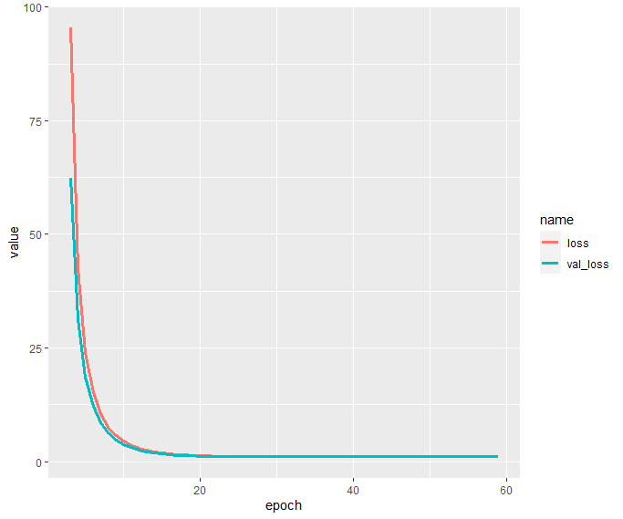
Interpretation via KernelSHAP
In order to peak into the fitted model, we apply the Kernel SHAP algorithm to decompose 500 randomly selected diamond predictions. We use the same subset as background dataset required by the Kernel SHAP algorithm.
Afterwards, we will study
- Some SHAP values and their standard errors
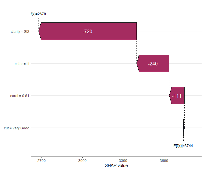
- One waterfall plot
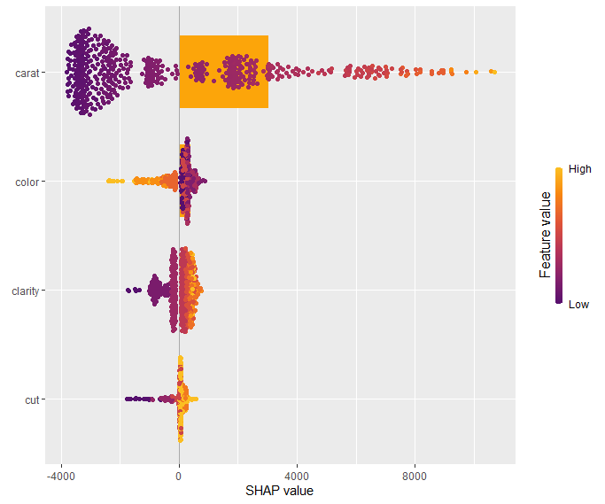
- A beeswarm summary plot to get a rough picture of variable importance and the direction of the feature effects
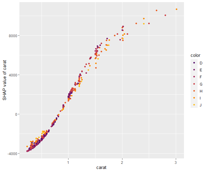
- A SHAP dependence plot for carat
# Interpretation on 500 randomly selected diamonds
library(kernelshap)
library(shapviz)

sample(1)
ind <- sample(nrow(X), 500)

dia_small <- X[ind, ]

# 77 seconds
system.time(
  ks <- kernelshap(
    dia_small,
    pred_fun = function(X) as.numeric(predict(nn, X, batch_size = nrow(X))),
    bg_X = dia_small
  )
)
ks

# Output
# 'kernelshap' object representing
# - SHAP matrix of dimension 500 x 4
# - feature data.frame/matrix of dimension 500 x 4
# - baseline value of 3744.153
#
# SHAP values of first 2 observations:
#         carat     color       cut   clarity
# [1,] -110.738 -240.2758  5.254733 -720.3610
# [2,] 2379.065  263.3112 56.413680  452.3044
#
# Corresponding standard errors:
#         carat      color       cut  clarity
# [1,] 2.064393 0.05113337 0.1374942 2.150754
# [2,] 2.614281 0.84934844 0.9373701 0.827563

sv <- shapviz(ks, X = diamonds[ind, x])
sv_waterfall(sv, 1)
sv_importance(sv, "both")
sv_dependence(sv, "carat", "auto")
Note the small standard errors of the SHAP values of the first two diamonds. They are only approximate because the background data is only a sample from an unknown population. Still, they give a good impression on the stability of the results.
The waterfall plot shows a diamond with not super nice clarity and color, pulling down the value of this diamond. Note that, even if the model is working with scaled numeric feature values, the plot shows the original feature values.
The SHAP summary plot shows that “carat” is, unsurprisingly, the most important variable and that high carat mean high value. “cut” is not very important, except if it is extremely bad.
Our last plot is a SHAP dependence plot for “carat”: the effect makes sense, and we can spot some interaction with color. For worse colors (H-J), the effect of carat is a bit less strong as for the very white diamonds.
Short wrap-up
- Standard Kernel SHAP in R, yeahhhhh 🙂
- The Github version is relatively fast, so you can even decompose 500 observations of a deep learning model within 1-2 minutes.
The complete R script can be found here.
Leave a Reply