It must have been around the year 2000, when I wrote my first snipped of SPLUS/R code. One thing I’ve learned back then:
Loops are slow. Replace them with
- vectorized calculations or
- if vectorization is not possible, use sapply() et al.
Since then, the R core team and the community has invested tons of time to improve R and also to make it faster. There are things like RCPP and parallel computing to speed up loops.
But what still relatively few R users know: loops are not that slow anymore. We want to demonstrate this using two examples.
Example 1: sqrt()
We use three ways to calculate the square root of a vector of random numbers:
- Vectorized calculation. This will be the way to go because it is internally optimized in C.
- A loop. This must be super slow for large vectors.
- vapply() (as safe alternative to sapply).
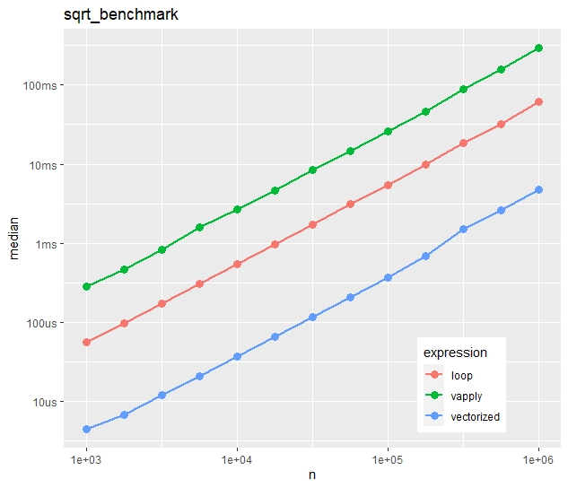
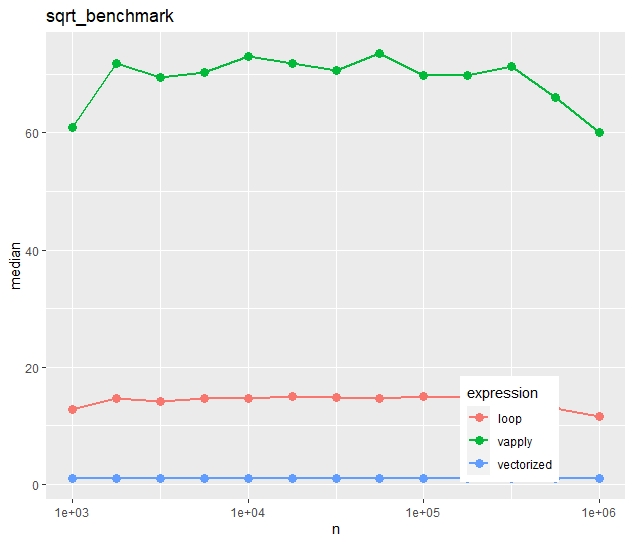
The three approaches are then compared via bench::mark() regarding their speed for different numbers n of vector lengths. The results are then compared first regarding absolute median times, and secondly (using an independent run), on a relative scale (1 is the vectorized approach).
library(tidyverse)
library(bench)

# Calculate square root for each element in loop
sqrt_loop <- function(x) {
  out <- numeric(length(x))
  for (i in seq_along(x)) {
    out[i] <- sqrt(x[i])
  }
  out
}

# Example
sqrt_loop(1:4) # 1.000000 1.414214 1.732051 2.000000

# Compare its performance with two alternatives
sqrt_benchmark <- function(n) {
  x <- rexp(n)
  mark(
    vectorized = sqrt(x),
    loop = sqrt_loop(x),
    vapply = vapply(x, sqrt, FUN.VALUE = 0.0),
    # relative = TRUE
  )
}

# Combine results of multiple benchmarks and plot results
multiple_benchmarks <- function(one_bench, N) {
  res <- vector("list", length(N))
  for (i in seq_along(N)) {
    res[[i]] <- one_bench(N[i]) %>%
      mutate(n = N[i], expression = names(expression))
  }

  ggplot(bind_rows(res), aes(n, median, color = expression)) +
    geom_point(size = 3) +
    geom_line(size = 1) +
    scale_x_log10() +
    ggtitle(deparse1(substitute(one_bench))) +
    theme(legend.position = c(0.8, 0.15))
}

# Apply simulation
multiple_benchmarks(sqrt_benchmark, N = 10^seq(3, 6, 0.25))
Absolute timings

Relative timings (using a second run)

We see:
- Run times increase quite linearly with vector size.
- Vectorization is more than ten times faster than the naive loop.
- Most strikingly, vapply() is much slower than the naive loop. Would you have thought this?
Example 2: paste()
For the second example, we use a less simple function, namely
paste(“Number”, prettyNum(x, digits = 5))
What will our three approaches (vectorized, naive loop, vapply) show on this task?
pretty_paste <- function(x) {
  paste("Number", prettyNum(x, digits = 5))
}

# Example
pretty_paste(pi) # "Number 3.1416"

# Again, call pretty_paste() for each element in a loop
paste_loop <- function(x) {
  out <- character(length(x))
  for (i in seq_along(x)) {
    out[i] <- pretty_paste(x[i])
  }
  out
}

# Compare its performance with two alternatives
paste_benchmark <- function(n) {
  x <- rexp(n)
  mark(
    vectorized = pretty_paste(x),
    loop = paste_loop(x),
    vapply = vapply(x, pretty_paste, FUN.VALUE = ""),
    # relative = TRUE
  )
}

multiple_benchmarks(paste_benchmark, N = 10^seq(3, 5, 0.25))
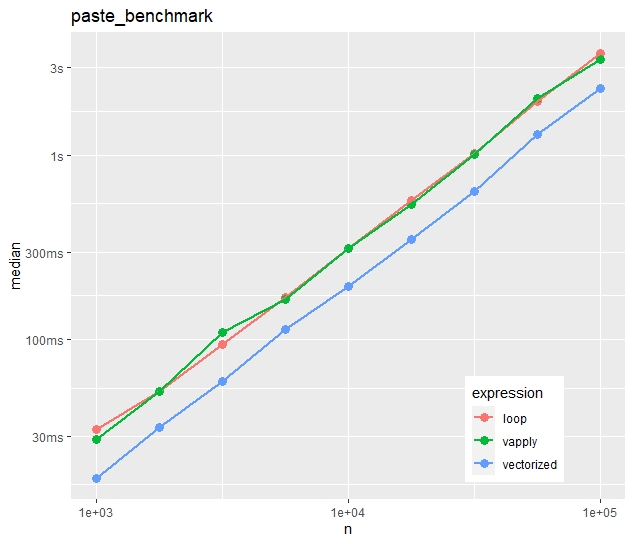
Absolute timings

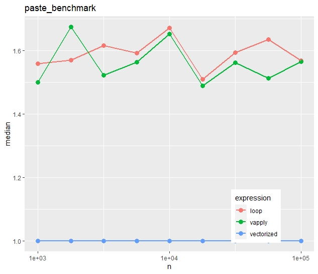
Relative timings (using a second run)

- In contrast to the first example, vapply() is now as fast as the naive loop.
- The time advantage of the vectorized approach is much less impressive. The loop takes in median only 50% longer.
Conclusion
- Vectorization is fast and easy to read. If available, use this. No surprise.
- If you use vapply/sapply/lapply, do it for the style, not for the speed. In some cases, the loop will be faster. And, depending on the situation and the audience, a loop might actually be even easier to read.
The code can be found on github.
The runs have been made on a Windows 11 system with a four core Intel(R) Core(TM) i7-8650U CPU @ 1.90GHz processor.
Leave a Reply