Tabular foundation models: simply a tool for impressing managers?

Or are they really worth having a look at?

Tabular data has had a comfortable life for years. Gradient boosting showed up, got very good at its job, and then quietly became the default answer to almost everything with rows and columns.

In very recent years, a new player has arrived: the tabular foundation model or prior fitted neural network, and suddenly tabular data is sounding a lot less sleepy…

Very roughly speaking: Such models have been pre-trained on data, where each observation consists of a synthetic dataset (X_train, y_train) with single response y_test corresponding to a single observation x_test. A specialized transformer neural net learns to study (X_train, y_train, x_test) to predict the conditional distribution of y_test as good as possible. Then, a new observation with a new synthetic dataset is generated, and the next iteration is done. The whole process is repeated millions of times. The secret sauce is how to generate the synthetic data to cover the nature of most data sets sufficiently well.

After being pre-trained, ideally, the model can look at your training data (X_train, Y_train) and sees: “hey, this data structure looks familiar, I know how to get predictions for that one”.

The best-known implementation is TabPFN. However in this post, I use tabicl from Inria because it is open source, has a permissive license, and is also extremely strong.

The goal of this blog post is not to bury gradient boosting. It is just to see whether tabular foundation models are a genuine new tool or just a trend that can be ignored.

Comparison with XGBoost on a real dataset

Let’s use a rich dataset with house prices of Miami, originally put together by Prof. Steven Bourassa. It has about 10k observations. The aim is to use a subset of the covariates to predict logarithmic prices.

Load data and build simple XGBoost model

We use a simple XGBoost regressor with default parameters as a strong baseline, using the validation data for early stopping to choose the number of trees.

import numpy as np
import shap
import xgboost as xgb
from sklearn.datasets import fetch_openml
from sklearn.metrics import mean_squared_error
from sklearn.model_selection import train_test_split


# Load data
df = fetch_openml(data_id=43093, as_frame=True)
X, y = df.data, np.log(df.target)

# Data split
x_vars = ["TOT_LVG_AREA", "LND_SQFOOT", "structure_quality", "age", "LONGITUDE", "LATITUDE"]

X_train, X_valid, y_train, y_valid = train_test_split(
    X[x_vars], y, test_size=0.2, random_state=30
)

# XGBoost baseline: fit with early stopping
dtrain = xgb.DMatrix(X_train, label=y_train)
dvalid = xgb.DMatrix(X_valid, label=y_valid)

params = {
    "learning_rate": 0.2,
    "objective": "reg:squarederror",
    "max_depth": 5,
}

xgb_model = xgb.train(
    params=params,
    dtrain=dtrain,
    evals=[(dvalid, "valid")],
    verbose_eval=20,
    early_stopping_rounds=20,
    num_boost_round=1000,
)

# Evaluate on validation
xgb_pred = xgb_model.predict(xgb.DMatrix(X_valid))
xgb_mse = mean_squared_error(y_valid, xgb_pred)
print(f"XGBoost validation RMSE: {np.sqrt(xgb_mse):.4}")  
# XGBoost validation RMSE: 0.1509

# SHAP analysis
xgb_shap_explainer = shap.Explainer(xgb_model)
xgb_shap_values = xgb_shap_explainer(X_valid)

shap.plots.bar(xgb_shap_values)
shap.plots.scatter(xgb_shap_values[:, "TOT_LVG_AREA"], color=xgb_shap_values)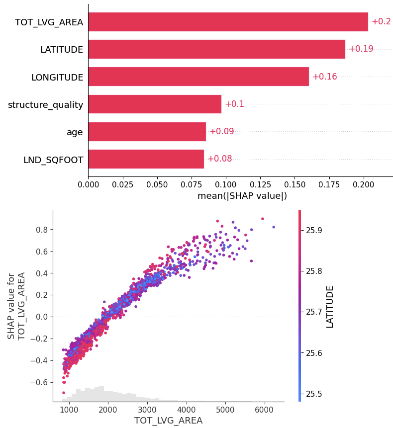

Now the prior fitted neural net

Note that we worked in Google Colab to have easy access to GPUs. Additionally, you need a Hugging Face access token to download the model weights of the pre-trained model. Many huggs to them for that beautiful hosting job.

from tabicl import TabICLRegressor

tabicl_model = TabICLRegressor(kv_cache=True, random_state=42)
tabicl_model.fit(X_train, y_train)  # Only data transformation is fitted, not the model

# Evaluate on validation data
tabicl_pred = tabicl_model.predict(X_valid)
tabicl_mse = mean_squared_error(y_valid, tabicl_pred)
print(f"TabICL validation RMSE: {np.sqrt(tabicl_mse):.4}")
# TabICL validation RMSE: 0.1311

# SHAP analysis
from tabicl.shap import get_shap_values, plot_shap, plot_shap_feature

tabicl_shap_values = get_shap_values(estimator=tabicl_model, X_test=X_valid[:200])
plot_shap(tabicl_shap_values)
plot_shap_feature(tabicl_shap_values, feature="TOT_LVG_AREA")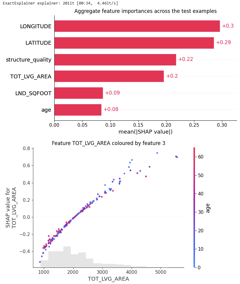

Comparison

1. Performance: Without any fine-tuning, the pre-trained model does substantially better than the slightly tuned XGBoost model: RMSE of 0.13 against 0.15. Wow!
2. Interpretation: TreeSHAP is zillion times faster and more reliable than running an exact permutation SHAP algorithm with a single background row. Still, its better than nothing. But there is room for improvement.
3. Ease of use: No fine-tuning, just .fit() and .predict(). However, we need some infrastructure (ideally GPU), and access to the model weights. Note that Inria provides tools to fine tune on your own data, which is absolutely insane. We will have a look at that in a later post.
4. Prediction intervals: Since tabular foundation models predict the full predictive posterior distribution for each observation (actually, a histogram), not only averages as in our example, but also medians or quartile (ranges) and therefore simple prediction intervals can be derived. Also this part I would like to cover later.
5. Limitations: There are many, e.g., we can’t use too big datasets or the SHAP values are not too realiable.

Just to impressing managers?

Nope. Even I as an absolute boosted tree lover am impressed 🙂

Jupyter notebook